How to visualize quantum circuit diagrams with Q#

Quantum circuit diagrams are a visual representation of quantum operations. Circuit diagrams show the flow of qubits through the quantum program, including the gates and measurements that the program applies to the qubits.

In this article, you learn how to visually represent quantum algorithms with quantum circuit diagrams in the Azure Quantum Development Kit (QDK) using Visual Studio Code (VS Code) and Jupyter Notebook.

For more information about quantum circuit diagrams, see Quantum circuit conventions.

Prerequisites

• The latest version of VS Code, or open VS Code for the Web.

• The latest version of the QDK extension, Python extension, and Jupyter extension installed in VS Code.

• The latest version of the qdk Python library with the optional jupyter extra.

  python -m pip install --upgrade qdk[jupyter]
  

Visualize quantum circuits in VS Code

To visualize quantum circuits of Q# programs in VS Code, complete the following steps.

View circuit diagrams for a Q# program

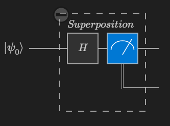
1. Open a Q# file in VS Code, or load one of the quantum samples.

2. Choose the Circuit command from the code lens that precedes your entry point operation.

   

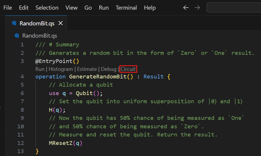
The Q# circuit window appears and displays the circuit diagram for your program. For example, the following circuit corresponds to an operation that puts a qubit in a superposition state and then measures the qubit. The circuit diagram shows one qubit register that's initialized to the $\ket{0}$ state. Then, a Hadamard gate is applied to the qubit, followed by a measurement operation, which is represented by a meter symbol. In this case, the measurement result is zero.

Tip

In Q# and OpenQASM files, select an element in the circuit diagram to highlight the code that creates the circuit element.

View circuit diagrams for individual operations

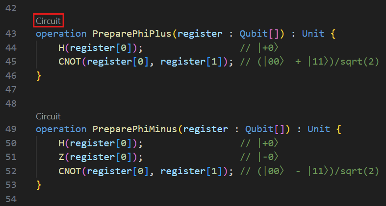
To visualize the quantum circuit for an individual operation in a Q# file, choose the Circuit command from the code lens that precedes the operation.

View circuit diagrams when you're debugging

When you use the VS Code debugger in a Q# program, you can visualize the quantum circuit based on the state of the program at the current debugger breakpoint.

1. Choose the Debug command from the code lens that precedes your entry point operation.
2. In the Run and Debug pane, expand the Quantum Circuit dropdown in the VARIABLES menu. The QDK Circuit panel opens, which shows the circuit while you step through the program.
3. Set breakpoints and step through your code to see how the circuit updates as your program runs.

Quantum circuits in Jupyter Notebook

In Jupyter Notebook, you can visualize quantum circuits with the qdk.qsharp and qdk.widgets Python modules. The widgets module provides a widget that renders a quantum circuit diagram as an SVG image.

View circuit diagrams for an entry expression

1. In VS Code, open the View menu and choose Command Palette.

2. Enter and select Create: New Jupyter Notebook.

3. In the first cell of the notebook, run the following code to import the qsharp package.

   from qdk import qsharp
   

4. Create a new cell and enter your Q# code. For example, the following code prepares a Bell State:

   %%qsharp
   
   // Prepare a Bell State.
   operation BellState() : Unit {
       use register = Qubit[2];
       H(register[0]);
       CNOT(register[0], register[1]);
   }
   

5. To display a simple quantum circuit based on the current state of your program, pass an entry point expression to the qsharp.circuit function. For example, the circuit diagram of the preceding code shows two qubit registers that are initialized to the $\ket{0}$ state. Then, a Hadamard gate is applied to the first qubit. Finally, a CNOT gate is applied where the first qubit is the control, represented by a dot, and the second qubit is the target, represented by an X.

   qsharp.circuit("BellState()")
   

   q_0    ── H ──── ● ──
   q_1    ───────── X ──
   

6. To visualize a quantum circuit as an SVG image, use the widgets module. Create a new cell, then run the following code to visualize the circuit that you created in the previous cell.

   from qdk.widgets import Circuit
   
   Circuit(qsharp.circuit("BellState()"))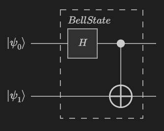
   

   

View circuit diagrams for operations with qubits

You can generate circuit diagrams of operations that take qubits, or arrays of qubits, as input. The diagram shows a wire for each input qubit, along with wires for additional qubits that you allocate within the operation. When the operation takes an array of qubits (Qubit[]), the circuit shows the array as a register of 2 qubits.

1. Add a new cell, and then copy and run the following Q# code. This code prepares a cat state.

   %%qsharp
   
   operation PrepareCatState(register : Qubit[]) : Unit {
       H(register[0]);
       ApplyToEach(CNOT(register[0], _), register[1...]);
   }
   

2. Add a new cell and run the following code to visualize the circuit of the PrepareCatState operation.

   Circuit(qsharp.circuit(operation="PrepareCatState"))
   

Circuit diagrams for dynamic circuits

Circuit diagrams are generated by executing the classical logic within a Q# program and keeping track of all allocated and applied gates. Loops and conditionals are supported when they deal only with classical values.

However, programs that contain loops and conditional expressions that use qubit measurement results are trickier to represent with a circuit diagram. For example, consider the following expression:

if (M(q) == One) {
   X(q)
}

This expression can't be represented with a straightforward circuit diagram because the gates are conditional on a measurement result. Circuits with gates that depend on measurement results are called dynamic circuits.

You can generate diagrams for dynamic circuits by running the program in the quantum simulator, and tracing the gates as they're applied. This is called trace mode because the qubits and gates are traced as the simulation is performed.

The downside of traced circuits is that they only capture the measurement outcome and the consequent gate applications for a single simulation. In the above example, if the measurement outcome is Zero, then the X gate isn't in the diagram. If you run the simulation again, then you might get a different circuit.