Simultaneous Localization and Mapping (SLAM) は、ロボットに必要な最も基本的な機能の 1 つです。 画像のユビキタスに利用できるため、Visual SLAM (V-SLAM) は多くの自律システムの重要なコンポーネントになりました。 幾何ベースの手法と学習ベースの手法の両方により、目覚ましい成長を遂げました。 しかし、実際のアプリケーションに対応する堅牢で信頼性の高い SLAM 手法を開発するには、まだ困難な課題があります。 現実の環境は、光源の変更や照明の不足、動的な物体、模様のないシーンなど、難しい事例であふれています。 このデータセットでは高度なコンピューター グラフィックス テクノロジが活用されており、シミュレーションでの魅力的な機能を使用して、さまざまなシナリオに対応できるようにすることを目的としています。
注
Microsoft は、Azure Open Datasets を "現状有姿" で提供します。 Microsoft は、データセットの使用に関して、明示または黙示を問わず、いかなる保証も行わないものとし、条件を定めることもありません。 現地の法律の下で認められている範囲内で、Microsoft は、データセットの使用に起因する、直接的、派生的、特別、間接的、偶発的、または懲罰的なものを含めたいかなる損害または損失に対しても一切の責任を負わないものとします。
このデータセットは、Microsoft がソース データを受け取った元の条件に基づいて提供されます。 データセットには、Microsoft が提供するデータが含まれている場合があります。
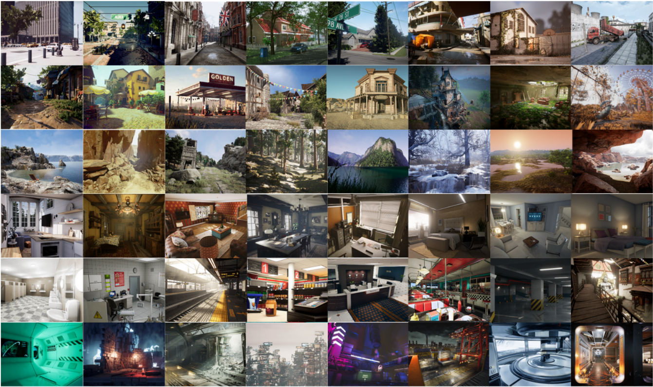
データはさまざまな光源の状態、気象、移動する物体などが存在するときのフォトリアリスティックなシミュレーション環境で収集されます。 シミュレーションでデータを収集することで、ステレオ RGB 画像、奥行き画像、セグメンテーション、オプティカル フロー、カメラ姿勢など、マルチモーダルのセンサー データや正確な Ground Truth ラベルを取得することができます。 物理的なデータ収集プラットフォームの使用では実現が難しい、実現が難しい視点やさまざまなモーション パターンに対応する、さまざまなスタイルやシーンの多数の環境をご用意しました。 データセットの最も重要な4つの特徴は、1) 大規模で多様な現実的データ、2) マルチモーダルなグラウンドトゥルースラベル、3) モーションパターンの多様性、4) 挑戦的なシーンです。
このデータセットは、次の 5 種類のデータを提供します。
- ステレオ イメージ: 画像型 (PNG)。
- 奥行ファイル: NumPy 型 (NPY)
- セグメンテーション ファイル: NumPy 型 (NPY)。
- オプティカル フロー ファイル: NumPy 型 (NPY)。
- カメラ姿勢ファイル: テキスト型 (TXT)。
これはさまざまな環境から収集され、2019 年時点で合計数百の軌道 (3 TB) が含まれています。
実現が難しいビジュアル効果
いくつかの状況では、データセットは複数の種類の実現が難しいビジュアル効果をシミュレートします。
- 難しい照明条件。 昼と夜の入れ替わり。 低い照度。 高速で変化するイルミネーション。
- 天候の影響。 晴れ、雨、雪、風、霧。
- 季節変化。
保存先
このデータセットは、米国東部 Azure リージョンに保存されています。 アフィニティを高めるために、米国東部でコンピューティング リソースを割り当てることをお勧めします。
ライセンス条項
このプロジェクトは MIT ライセンスの下でリリースされました。 詳細については、ライセンス ファイルを確認してください。
追加情報
TartanAir の公式 Web サイトを参照するか、元の研究論文を参照してください。
データ ソースについてご不明な点があれば、tartanair@hotmail.com までメールでお問い合わせください。 関連する GitHub で共同作成者に連絡することもできます。
引用: より技術的な詳細については、AirSim の論文 (FSR 2017 Conference) を参照してください。 これを次のように引用します。
@article{tartanair2020arxiv,
  title =   {TartanAir: A Dataset to Push the Limits of Visual SLAM},
  author =  {Wenshan Wang, Delong Zhu, Xiangwei Wang, Yaoyu Hu, Yuheng Qiu, Chen Wang, Yafei Hu, Ashish Kapoor, Sebastian Scherer},
  journal = {arXiv preprint arXiv:2003.14338},
  year =    {2020},
  url = {https://arxiv.org/abs/2003.14338}
}
@inproceedings{airsim2017fsr,
  author = {Shital Shah and Debadeepta Dey and Chris Lovett and Ashish Kapoor},
  title = {AirSim: High-Fidelity Visual and Physical Simulation for Autonomous Vehicles},
  year = {2017},
  booktitle = {Field and Service Robotics},
  eprint = {arXiv:1705.05065},
  url = {https://arxiv.org/abs/1705.05065}
}
データ アクセス
Python ノートブックのデータにアクセスするには、次のコード サンプルを使用します。
依存関係
pip install numpy
pip install azure-storage-blob
pip install opencv-python
インポートとコンテナー クライアント
from azure.storage.blob import ContainerClient
import numpy as np
import io
import cv2
import time
import matplotlib.pyplot as plt
%matplotlib inline

# Dataset website: http://theairlab.org/tartanair-dataset/
account_url = 'https://tartanair.blob.core.windows.net/'
container_name = 'tartanair-release1'

container_client = ContainerClient(account_url=account_url,
                                 container_name=container_name,
                                 credential=None)
環境と軌道
def get_environment_list():
    '''
    List all the environments shown in the root directory
    '''
    env_gen = container_client.walk_blobs()
    envlist = []
    for env in env_gen:
        envlist.append(env.name)
    return envlist

def get_trajectory_list(envname, easy_hard = 'Easy'):
    '''
    List all the trajectory folders, which is named as 'P0XX'
    '''
    assert(easy_hard=='Easy' or easy_hard=='Hard')
    traj_gen = container_client.walk_blobs(name_starts_with=envname + '/' + easy_hard+'/')
    trajlist = []
    for traj in traj_gen:
        trajname = traj.name
        trajname_split = trajname.split('/')
        trajname_split = [tt for tt in trajname_split if len(tt)>0]
        if trajname_split[-1][0] == 'P':
            trajlist.append(trajname)
    return trajlist

def _list_blobs_in_folder(folder_name):
    """
    List all blobs in a virtual folder in an Azure blob container
    """

    files = []
    generator = container_client.list_blobs(name_starts_with=folder_name)
    for blob in generator:
        files.append(blob.name)
    return files

def get_image_list(trajdir, left_right = 'left'):
    assert(left_right == 'left' or left_right == 'right')
    files = _list_blobs_in_folder(trajdir + '/image_' + left_right + '/')
    files = [fn for fn in files if fn.endswith('.png')]
    return files

def get_depth_list(trajdir, left_right = 'left'):
    assert(left_right == 'left' or left_right == 'right')
    files = _list_blobs_in_folder(trajdir + '/depth_' + left_right + '/')
    files = [fn for fn in files if fn.endswith('.npy')]
    return files

def get_flow_list(trajdir, ):
    files = _list_blobs_in_folder(trajdir + '/flow/')
    files = [fn for fn in files if fn.endswith('flow.npy')]
    return files

def get_flow_mask_list(trajdir, ):
    files = _list_blobs_in_folder(trajdir + '/flow/')
    files = [fn for fn in files if fn.endswith('mask.npy')]
    return files

def get_posefile(trajdir, left_right = 'left'):
    assert(left_right == 'left' or left_right == 'right')
    return trajdir + '/pose_' + left_right + '.txt'

def get_seg_list(trajdir, left_right = 'left'):
    assert(left_right == 'left' or left_right == 'right')
    files = _list_blobs_in_folder(trajdir + '/seg_' + left_right + '/')
    files = [fn for fn in files if fn.endswith('.npy')]
    return files
環境の一覧表示
envlist = get_environment_list()
print('Find {} environments..'.format(len(envlist)))
print(envlist)
最初の環境での "Easy" 軌道の一覧表示
diff_level = 'Easy'
env_ind = 0
trajlist = get_trajectory_list(envlist[env_ind], easy_hard = diff_level)
print('Find {} trajectories in {}'.format(len(trajlist), envlist[env_ind]+diff_level))
print(trajlist)
1 つの軌道のすべてのデータ ファイルの一覧表示
traj_ind = 1
traj_dir = trajlist[traj_ind]

left_img_list = get_image_list(traj_dir, left_right = 'left')
print('Find {} left images in {}'.format(len(left_img_list), traj_dir))

right_img_list = get_image_list(traj_dir, left_right = 'right')
print('Find {} right images in {}'.format(len(right_img_list), traj_dir))

left_depth_list = get_depth_list(traj_dir, left_right = 'left')
print('Find {} left depth files in {}'.format(len(left_depth_list), traj_dir))

right_depth_list = get_depth_list(traj_dir, left_right = 'right')
print('Find {} right depth files in {}'.format(len(right_depth_list), traj_dir))

left_seg_list = get_seg_list(traj_dir, left_right = 'left')
print('Find {} left segmentation files in {}'.format(len(left_seg_list), traj_dir))

right_seg_list = get_seg_list(traj_dir, left_right = 'left')
print('Find {} right segmentation files in {}'.format(len(right_seg_list), traj_dir))

flow_list = get_flow_list(traj_dir)
print('Find {} flow files in {}'.format(len(flow_list), traj_dir))

flow_mask_list = get_flow_mask_list(traj_dir)
print('Find {} flow mask files in {}'.format(len(flow_mask_list), traj_dir))

left_pose_file = get_posefile(traj_dir, left_right = 'left')
print('Left pose file: {}'.format(left_pose_file))

right_pose_file = get_posefile(traj_dir, left_right = 'right')
print('Right pose file: {}'.format(right_pose_file))
データ ダウンロード関数
def read_numpy_file(numpy_file,):
    '''
    return a numpy array given the file path
    '''
    bc = container_client.get_blob_client(blob=numpy_file)
    data = bc.download_blob()
    ee = io.BytesIO(data.content_as_bytes())
    ff = np.load(ee)
    return ff


def read_image_file(image_file,):
    '''
    return a uint8 numpy array given the file path
    '''
    bc = container_client.get_blob_client(blob=image_file)
    data = bc.download_blob()
    ee = io.BytesIO(data.content_as_bytes())
    img=cv2.imdecode(np.asarray(bytearray(ee.read()),dtype=np.uint8), cv2.IMREAD_COLOR)
    im_rgb = img[:, :, [2, 1, 0]] # BGR2RGB
    return im_rgb
データ視覚化関数
def depth2vis(depth, maxthresh = 50):
    depthvis = np.clip(depth,0,maxthresh)
    depthvis = depthvis/maxthresh*255
    depthvis = depthvis.astype(np.uint8)
    depthvis = np.tile(depthvis.reshape(depthvis.shape+(1,)), (1,1,3))

    return depthvis

def seg2vis(segnp):
    colors = [(205, 92, 92), (0, 255, 0), (199, 21, 133), (32, 178, 170), (233, 150, 122), (0, 0, 255), (128, 0, 0), (255, 0, 0), (255, 0, 255), (176, 196, 222), (139, 0, 139), (102, 205, 170), (128, 0, 128), (0, 255, 255), (0, 255, 255), (127, 255, 212), (222, 184, 135), (128, 128, 0), (255, 99, 71), (0, 128, 0), (218, 165, 32), (100, 149, 237), (30, 144, 255), (255, 0, 255), (112, 128, 144), (72, 61, 139), (165, 42, 42), (0, 128, 128), (255, 255, 0), (255, 182, 193), (107, 142, 35), (0, 0, 128), (135, 206, 235), (128, 0, 0), (0, 0, 255), (160, 82, 45), (0, 128, 128), (128, 128, 0), (25, 25, 112), (255, 215, 0), (154, 205, 50), (205, 133, 63), (255, 140, 0), (220, 20, 60), (255, 20, 147), (95, 158, 160), (138, 43, 226), (127, 255, 0), (123, 104, 238), (255, 160, 122), (92, 205, 92),]
    segvis = np.zeros(segnp.shape+(3,), dtype=np.uint8)

    for k in range(256):
        mask = segnp==k
        colorind = k % len(colors)
        if np.sum(mask)>0:
            segvis[mask,:] = colors[colorind]

    return segvis

def _calculate_angle_distance_from_du_dv(du, dv, flagDegree=False):
    a = np.arctan2( dv, du )

    angleShift = np.pi

    if ( True == flagDegree ):
        a = a / np.pi * 180
        angleShift = 180
        # print("Convert angle from radian to degree as demanded by the input file.")

    d = np.sqrt( du * du + dv * dv )

    return a, d, angleShift

def flow2vis(flownp, maxF=500.0, n=8, mask=None, hueMax=179, angShift=0.0):
    """
    Show an optical flow field as the KITTI dataset does.
    Some parts of this function is the transform of the original MATLAB code flow_to_color.m.
    """

    ang, mag, _ = _calculate_angle_distance_from_du_dv( flownp[:, :, 0], flownp[:, :, 1], flagDegree=False )

    # Use Hue, Saturation, Value colour model
    hsv = np.zeros( ( ang.shape[0], ang.shape[1], 3 ) , dtype=np.float32)

    am = ang < 0
    ang[am] = ang[am] + np.pi * 2

    hsv[ :, :, 0 ] = np.remainder( ( ang + angShift ) / (2*np.pi), 1 )
    hsv[ :, :, 1 ] = mag / maxF * n
    hsv[ :, :, 2 ] = (n - hsv[:, :, 1])/n

    hsv[:, :, 0] = np.clip( hsv[:, :, 0], 0, 1 ) * hueMax
    hsv[:, :, 1:3] = np.clip( hsv[:, :, 1:3], 0, 1 ) * 255
    hsv = hsv.astype(np.uint8)

    rgb = cv2.cvtColor(hsv, cv2.COLOR_HSV2RGB)

    if ( mask is not None ):
        mask = mask > 0
        rgb[mask] = np.array([0, 0 ,0], dtype=np.uint8)

    return rgb
ダウンロードと視覚化
data_ind = 173 # randomly select one frame (data_ind < TRAJ_LEN)

left_img = read_image_file(left_img_list[data_ind])
right_img = read_image_file(right_img_list[data_ind])

# Visualize the left and right RGB images
plt.figure(figsize=(12, 5))
plt.subplot(121)
plt.imshow(left_img)
plt.title('Left Image')
plt.subplot(122)
plt.imshow(right_img)
plt.title('Right Image')
plt.show()

# Visualize the left and right depth files
left_depth = read_numpy_file(left_depth_list[data_ind])
left_depth_vis = depth2vis(left_depth)

right_depth = read_numpy_file(right_depth_list[data_ind])
right_depth_vis = depth2vis(right_depth)

plt.figure(figsize=(12, 5))
plt.subplot(121)
plt.imshow(left_depth_vis)
plt.title('Left Depth')
plt.subplot(122)
plt.imshow(right_depth_vis)
plt.title('Right Depth')
plt.show()

# Visualize the left and right segmentation files
left_seg = read_numpy_file(left_seg_list[data_ind])
left_seg_vis = seg2vis(left_seg)

right_seg = read_numpy_file(right_seg_list[data_ind])
right_seg_vis = seg2vis(right_seg)

plt.figure(figsize=(12, 5))
plt.subplot(121)
plt.imshow(left_seg_vis)
plt.title('Left Segmentation')
plt.subplot(122)
plt.imshow(right_seg_vis)
plt.title('Right Segmentation')
plt.show()

# Visualize the flow and mask files

flow = read_numpy_file(flow_list[data_ind])
flow_vis = flow2vis(flow)

flow_mask = read_numpy_file(flow_mask_list[data_ind])
flow_vis_w_mask = flow2vis(flow, mask = flow_mask)

plt.figure(figsize=(12, 5))
plt.subplot(121)
plt.imshow(flow_vis)
plt.title('Optical Flow')
plt.subplot(122)
plt.imshow(flow_vis_w_mask)
plt.title('Optical Flow w/ Mask')
plt.show()
次のステップ
Open Datasets カタログの残りのデータセットを表示します。