このチュートリアルでは、Microsoft Fabric の Synapse Data Science ワークフローのエンド ツー エンドの例を示します。 このシナリオでは、履歴データでトレーニングされた機械学習アルゴリズムを使用して、R で不正検出モデルを構築します。 次に、このモデルを使用して、将来の不正なトランザクションを検出します。
このチュートリアルでは、次の手順について説明します。
- カスタム ライブラリをインストールする
- データを読み込む
- 探索的データ分析を使用してデータを理解して処理し、Fabric Data Wrangler 機能の使用を示す
- LightGBM を使用して機械学習モデルをトレーニングする
- スコアリングと予測に機械学習モデルを使用する
前提 条件
Microsoft Fabric サブスクリプションを取得します。 または、無料の Microsoft Fabric 試用版にサインアップします。
Microsoft Fabric にサインインします。
ホーム ページの左下にあるエクスペリエンス スイッチャーを使用して、Fabric に切り替えます。
- 必要に応じて、「Microsoft Fabric でレイクハウスを作成する」で説明されているように、Microsoft Fabric レイクハウスを作成します。
ノートブックで作業を進める
ノートブックでご利用いただける次のいずれかのオプションを選べます。
- Synapse Data Science エクスペリエンスで組み込みのノートブックを開いて実行する
- GitHub から Synapse Data Science エクスペリエンスにノートブックをアップロードする
組み込みのノートブックを開く
サンプルの不正行為の検出ノートブックが、このチュートリアルに付属しています。
チュートリアルのサンプルノートブックを開くには、「データサイエンス用にシステムを準備する」の手順に従ってください。。
コードの実行を開始する前に、必ずレイクハウスをノートブックにアタッチしてください。
GitHub からノートブックをインポートする
このチュートリアルには、AIsample - R Fraud Detection.ipynb ノートブックが付属しています。
このチュートリアルの付属のノートブックを開くには、「データ サイエンス用にシステムを準備する」の手順に従って、ノートブックをワークスペースにインポート します。
新しいノートブック を作成する場合は、このページからコードをコピーして貼り付けることができます。
コードを実行する前に、必ずノートブック にレイクハウス をアタッチしてください。
手順 1: カスタム ライブラリをインストールする
機械学習モデルの開発やアドホック データ分析の場合は、Apache Spark セッション用のカスタム ライブラリをすばやくインストールすることが必要になる場合があります。 ライブラリをインストールするには、2 つのオプションがあります。
- 現在のノートブックにのみインストールするには、インライン インストール リソース (
install.packagesやdevtools::install_versionなど) を使用します。 - または、ファブリック環境を作成したり、パブリック ソースからライブラリをインストールしたり、カスタム ライブラリをアップロードしたりして、ワークスペース管理者がワークスペースの既定として環境をアタッチすることもできます。 その後、環境内のすべてのライブラリが、ワークスペース内のすべてのノートブックと Spark ジョブ定義で使用できるようになります。 環境の詳細については、「Microsoft Fabric で環境作成、構成、および使用する」を参照してください。
このチュートリアルでは、install.version() を使用して、不均衡な learn ライブラリをインストールします。
# Install dependencies
devtools::install_version("bnlearn", version = "4.8")
# Install imbalance for SMOTE
devtools::install_version("imbalance", version = "1.0.2.1")
手順 2: データを読み込む
不正検出データセットには、2013 年 9 月のクレジット カード トランザクションが含まれています。このトランザクションは、ヨーロッパのカード所有者が 2 日間にわたって行いました。 データセットには、元のフィーチャに適用された主成分分析 (PCA) 変換が原因で、数値特徴のみが含まれます。 PCA は、Time と Amountを除くすべての機能を変換しました。 機密性を保護するために、データセットに関する元の機能や背景情報を提供することはできません。
これらの詳細では、データセットについて説明します。
V1、V2、V3、...、V28機能は、PCA で取得された主要コンポーネントですTime機能には、トランザクションとデータセット内の最初のトランザクションの間の経過時間 (秒) が含まれていますAmount機能はトランザクション量です。 この機能は、たとえば、コスト重視の学習に使用できます。Class列は応答 (ターゲット) 変数です。 不正行為の場合は値1を持ち、それ以外の場合は0を持ちます。
284,807 件のトランザクションのうち、不正なトランザクションは 492 件のみです。 少数派 (不正) クラスはデータの約 0.172% のみを占めるので、データセットは非常に不均衡です。
次の表に、creditcard.csv データのプレビューを示します。
| 時間 | V1 | V2 | V3 | V4 | V5 | V6 | V7 | V8 | V9 | V10 | V11 | V12 | V13 | V14 | V15 | V16 | V17 | V18 | V19 | V20 | V21 | V22 | V23 | V24 | V25 | V26 | V27 | V28 | 金額 | クラス |
|---|---|---|---|---|---|---|---|---|---|---|---|---|---|---|---|---|---|---|---|---|---|---|---|---|---|---|---|---|---|---|
| 0 | -1.3598071336738 | -0.0727811733098497 | 2.53634673796914 | 1.37815522427443 | -0.338320769942518 | 0.462387777762292 | 0.239598554061257 | 0.0986979012610507 | 0.363786969611213 | 0.0907941719789316 | -0.551599533260813 | -0.617800855762348 | -0.991389847235408 | -0.311169353699879 | 1.46817697209427 | -0.470400525259478 | 0.207971241929242 | 0.0257905801985591 | 0.403992960255733 | 0.251412098239705 | -0.018306777944153 | 0.277837575558899 | -0.110473910188767 | 0.0669280749146731 | 0.128539358273528 | -0.189114843888824 | 0.133558376740387 | -0.0210530534538215 | 149.62 | "0" |
| 0 | 1.19185711131486 | 0.26615071205963 | 0.16648011335321 | 0.448154078460911 | 0.0600176492822243 | -0.0823608088155687 | -0.0788029833323113 | 0.0851016549148104 | -0.255425128109186 | -0.166974414004614 | 1.61272666105479 | 1.06523531137287 | 0.48909501589608 | -0.143772296441519 | 0.635558093258208 | 0.463917041022171 | -0.114804663102346 | -0.183361270123994 | -0.145783041325259 | -0.0690831352230203 | -0.225775248033138 | -0.638671952771851 | 0.101288021253234 | -0.339846475529127 | 0.167170404418143 | 0.125894532368176 | -0.00898309914322813 | 0.0147241691924927 | 2.69 | "0" |
データセットをダウンロードして lakehouse にアップロードする
さまざまなデータセットでこのノートブックを使用できるように、これらのパラメーターを定義します。
IS_CUSTOM_DATA <- FALSE  # If TRUE, the dataset has to be uploaded manually

IS_SAMPLE <- FALSE  # If TRUE, use only rows of data for training; otherwise, use all data
SAMPLE_ROWS <- 5000  # If IS_SAMPLE is True, use only this number of rows for training

DATA_ROOT <- "/lakehouse/default"
DATA_FOLDER <- "Files/fraud-detection"  # Folder with data files
DATA_FILE <- "creditcard.csv"  # Data file name
このコードは、公開されているバージョンのデータセットをダウンロードし、Fabric Lakehouse に格納します。
重要
実行する前にノートブックにレイクハウスを追加してください。 それ以外の場合は、エラーが発生します。
if (!IS_CUSTOM_DATA) {
    # Download data files into a lakehouse if they don't exist
    library(httr)

    remote_url <- "https://synapseaisolutionsa.blob.core.windows.net/public/Credit_Card_Fraud_Detection"
    fname <- "creditcard.csv"
    download_path <- file.path(DATA_ROOT, DATA_FOLDER, "raw")

    dir.create(download_path, showWarnings = FALSE, recursive = TRUE)
    if (!file.exists(file.path(download_path, fname))) {
        r <- GET(file.path(remote_url, fname), timeout(30))
        writeBin(content(r, "raw"), file.path(download_path, fname))
    }
    message("Downloaded demo data files into lakehouse.")
}
レイクハウスから日付の生データを読み取る
このコードは、lakehouse の Files セクションから生データを読み取ります。
data_df <- read.csv(file.path(DATA_ROOT, DATA_FOLDER, "raw", DATA_FILE))
手順 3: 探索的データ分析を実行する
display コマンドを使用して、データセットの高度な統計情報を表示します。
display(as.DataFrame(data_df, numPartitions = 3L))
# Print dataset basic information
message(sprintf("records read: %d", nrow(data_df)))
message("Schema:")
str(data_df)
# If IS_SAMPLE is True, use only SAMPLE_ROWS of rows for training
if (IS_SAMPLE) {
    data_df = sample_n(data_df, SAMPLE_ROWS)
}
データセット内のクラスの分布を出力します。
# The distribution of classes in the dataset
message(sprintf("No Frauds %.2f%% of the dataset\n", round(sum(data_df$Class == 0)/nrow(data_df) * 100, 2)))
message(sprintf("Frauds %.2f%% of the dataset\n", round(sum(data_df$Class == 1)/nrow(data_df) * 100, 2)))
このクラス分布は、ほとんどのトランザクションが不正行為ではないことを示しています。 そのため、オーバーフィットを回避するには、モデルトレーニングの前にデータの前処理が必要です。
不正なトランザクションと正当なトランザクションの分布を表示する
プロットを使用して不正トランザクションと非侵害トランザクションの分布を表示し、データセット内のクラスの不均衡を表示します。
library(ggplot2)

ggplot(data_df, aes(x = factor(Class), fill = factor(Class))) +
  geom_bar(stat = "count") +
  scale_x_discrete(labels = c("no fraud", "fraud")) +
  ggtitle("Class Distributions \n (0: No Fraud || 1: Fraud)") +
  theme(plot.title = element_text(size = 10))
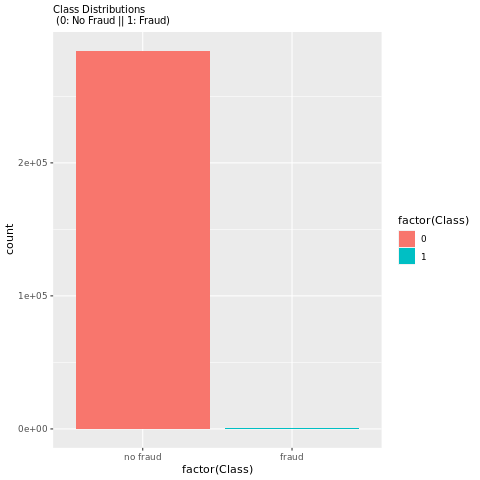
プロットには、データセットの不均衡が明確に示されています。
5 つの数値の概要を表示する
取引金額の 5 つの数値の概要 (最小スコア、最初の四分位数、中央値、3 番目の四分位数、および最大スコア) をボックス プロットと共に表示します。
library(ggplot2)
library(dplyr)

ggplot(data_df, aes(x = as.factor(Class), y = Amount, fill = as.factor(Class))) +
  geom_boxplot(outlier.shape = NA) +
  scale_x_discrete(labels = c("no fraud", "fraud")) +
  ggtitle("Boxplot without Outliers") +
  coord_cartesian(ylim = quantile(data_df$Amount, c(0.05, 0.95)))
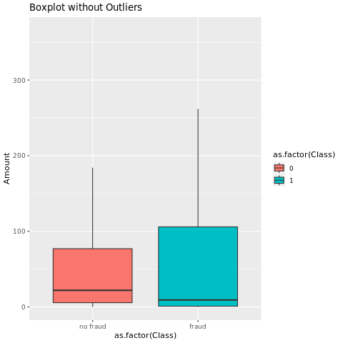
非常に不均衡なデータの場合、箱ひげ図では正確な分析情報が表示されない場合があります。 ただし、最初に Class 不均衡の問題に対処してから、より正確な分析情報を得るための同じプロットを作成できます。
手順 4: モデルをトレーニングして評価する
ここでは、不正取引を分類する LightGBM モデルをトレーニングします。 不均衡なデータセットとバランスの取れたデータセットの両方で LightGBM モデルをトレーニングします。 次に、両方のモデルのパフォーマンスを比較します。
トレーニング データセットとテスト データセットを準備する
トレーニングの前に、データをトレーニング データセットとテスト データセットに分割します。
# Split the dataset into training and test datasets
set.seed(42)
train_sample_ids <- base::sample(seq_len(nrow(data_df)), size = floor(0.85 * nrow(data_df)))

train_df <- data_df[train_sample_ids, ]
test_df <- data_df[-train_sample_ids, ]
トレーニング データセットに SMOTE を適用する
不均衡な分類には問題があります。 モデルが決定境界を効果的に学習するには、少数派クラスの例が少なすぎます。 合成少数派オーバーサンプリング手法 (SMOTE) は、この問題を処理できます。 SMOTE は、少数派クラスの新しいサンプルを合成するために最も広く使用されているアプローチです。 SMOTE には、手順 1 でインストールした imbalance ライブラリを使用してアクセスできます。
テスト データセットではなく、トレーニング データセットにのみ SMOTE を適用します。 テスト データを使用してモデルにスコアを付ける場合は、運用環境で見えないデータに対するモデルのパフォーマンスの近似値が必要です。 有効な近似値を得るために、テスト データは元の不均衡な分布に依存して、運用環境のデータを可能な限り厳密に表します。
# Apply SMOTE to the training dataset
library(imbalance)

# Print the shape of the original (imbalanced) training dataset
train_y_categ <- train_df %>% select(Class) %>% table
message(
    paste0(
        "Original dataset shape ",
        paste(names(train_y_categ), train_y_categ, sep = ": ", collapse = ", ")
    )
)

# Resample the training dataset by using SMOTE
smote_train_df <- train_df %>%
    mutate(Class = factor(Class)) %>%
    oversample(ratio = 0.99, method = "SMOTE", classAttr = "Class") %>%
    mutate(Class = as.integer(as.character(Class)))

# Print the shape of the resampled (balanced) training dataset
smote_train_y_categ <- smote_train_df %>% select(Class) %>% table
message(
    paste0(
        "Resampled dataset shape ",
        paste(names(smote_train_y_categ), smote_train_y_categ, sep = ": ", collapse = ", ")
    )
)
SMOTE の詳細については、CRAN Web サイトの パッケージ「imbalance」 と 不均衡データセットの取り扱いに関する リソースを参照してください。
LightGBM を使用してモデルをトレーニングする
不均衡なデータセットとバランスの取れた (SMOTE を介した) データセットの両方を使用して、LightGBM モデルをトレーニングします。 次に、パフォーマンスを比較します。
# Train LightGBM for both imbalanced and balanced datasets and define the evaluation metrics
library(lightgbm)

# Get the ID of the label column
label_col <- which(names(train_df) == "Class")

# Convert the test dataset for the model
test_mtx <- as.matrix(test_df)
test_x <- test_mtx[, -label_col]
test_y <- test_mtx[, label_col]

# Set up the parameters for training
params <- list(
    objective = "binary",
    learning_rate = 0.05,
    first_metric_only = TRUE
)

# Train for the imbalanced dataset
message("Start training with imbalanced data:")
train_mtx <- as.matrix(train_df)
train_x <- train_mtx[, -label_col]
train_y <- train_mtx[, label_col]
train_data <- lgb.Dataset(train_x, label = train_y)
valid_data <- lgb.Dataset.create.valid(train_data, test_x, label = test_y)
model <- lgb.train(
    data = train_data,
    params = params,
    eval = list("binary_logloss", "auc"),
    valids = list(valid = valid_data),
    nrounds = 300L
)

# Train for the balanced (via SMOTE) dataset
message("\n\nStart training with balanced data:")
smote_train_mtx <- as.matrix(smote_train_df)
smote_train_x <- smote_train_mtx[, -label_col]
smote_train_y <- smote_train_mtx[, label_col]
smote_train_data <- lgb.Dataset(smote_train_x, label = smote_train_y)
smote_valid_data <- lgb.Dataset.create.valid(smote_train_data, test_x, label = test_y)
smote_model <- lgb.train(
    data = smote_train_data,
    params = params,
    eval = list("binary_logloss", "auc"),
    valids = list(valid = smote_valid_data),
    nrounds = 300L
)
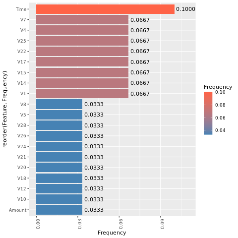
特徴の重要度を決定する
不均衡なデータセットでトレーニングしたモデルの特徴量の重要度を決定します。
imp <- lgb.importance(model, percentage = TRUE)
ggplot(imp, aes(x = Frequency, y = reorder(Feature, Frequency), fill = Frequency)) +
  scale_fill_gradient(low="steelblue", high="tomato") +
  geom_bar(stat = "identity") +
  geom_text(aes(label = sprintf("%.4f", Frequency)), hjust = -0.1) +
  theme(axis.text.x = element_text(angle = 90)) +
  xlim(0, max(imp$Frequency) * 1.1)
SMOTEでバランスをとったデータセットでトレーニングしたモデルについて、特徴量の重要度を計算します。
smote_imp <- lgb.importance(smote_model, percentage = TRUE)
ggplot(smote_imp, aes(x = Frequency, y = reorder(Feature, Frequency), fill = Frequency)) +
  geom_bar(stat = "identity") +
  scale_fill_gradient(low="steelblue", high="tomato") +
  geom_text(aes(label = sprintf("%.4f", Frequency)), hjust = -0.1) +
  theme(axis.text.x = element_text(angle = 90)) +
  xlim(0, max(smote_imp$Frequency) * 1.1)
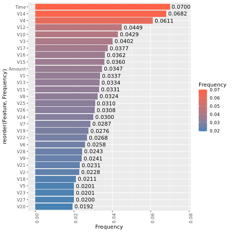
これらのプロットを比較すると、バランスの取れたトレーニング データセットと不均衡なトレーニング データセットには、特徴の重要度の違いが大きいことが明確に示されています。
モデルを評価する
ここでは、トレーニング済みの 2 つのモデルを評価します。
- 未加工で不均衡なデータをもとにトレーニングされた
model smote_modelはバランスの取れたデータに対してトレーニング済み
preds <- predict(model, test_mtx[, -label_col])
smote_preds <- predict(smote_model, test_mtx[, -label_col])
混同行列を使用してモデルのパフォーマンスを評価する
"混同行列" に以下の数が表示されます
- 真陽性 (TP)
- 真陰性 (TN)
- 偽陽性 (FP)
- 偽陰性 (FN)
モデルがテストデータでスコア付けされた時に生成する 二項分類の場合、モデルは 2x2 混同行列を返します。 多クラス分類の場合、モデルは nxn 混同行列を返します。ここで、n はクラスの数です。
混同行列を使用して、トレーニング済みの機械学習モデルのテスト データのパフォーマンスを要約します。
plot_cm <- function(preds, refs, title) {
    library(caret)
    cm <- confusionMatrix(factor(refs), factor(preds))
    cm_table <- as.data.frame(cm$table)
    cm_table$Prediction <- factor(cm_table$Prediction, levels=rev(levels(cm_table$Prediction)))

    ggplot(cm_table, aes(Reference, Prediction, fill = Freq)) +
            geom_tile() +
            geom_text(aes(label = Freq)) +
            scale_fill_gradient(low = "white", high = "steelblue", trans = "log") +
            labs(x = "Prediction", y = "Reference", title = title) +
            scale_x_discrete(labels=c("0", "1")) +
            scale_y_discrete(labels=c("1", "0")) +
            coord_equal() +
            theme(legend.position = "none")
}
不均衡なデータセットでトレーニングされたモデルの混同行列をプロットします。
# The value of the prediction indicates the probability that a transaction is fraud
# Use 0.5 as the threshold for fraud/no-fraud transactions
plot_cm(ifelse(preds > 0.5, 1, 0), test_df$Class, "Confusion Matrix (Imbalanced dataset)")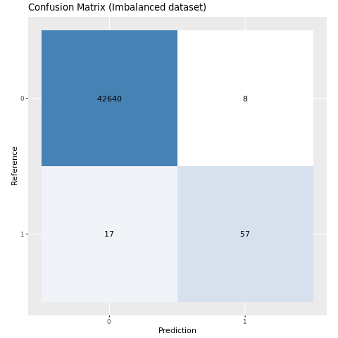
バランスの取れたデータセットでトレーニングされたモデルの混同行列をプロットします。
plot_cm(ifelse(smote_preds > 0.5, 1, 0), test_df$Class, "Confusion Matrix (Balanced dataset)")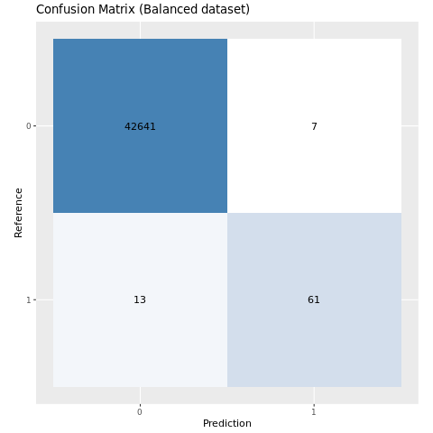
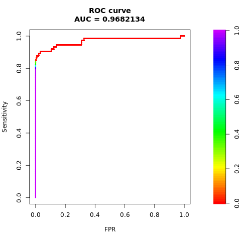
AUC-ROC と AUPRC 指標を使用してモデルのパフォーマンスを評価する
曲線レシーバ動作特性下面積(AUC-ROC)測定は、二項分類子のパフォーマンスを評価します。 AUC-ROC グラフでは、真陽性率 (TPR) と偽陽性率 (FPR) の間のトレードオフが視覚化されます。
場合によっては、Precision-Recall 曲線下面積 (AUPRC) 指標に基づいて分類器を評価する方が適切です。 AUPRC 曲線では、次のレートが結合されます。
- 精度、または正の予測値 (PPV)
- リコールまたは TPR
# Use the PRROC package to help calculate and plot AUC-ROC and AUPRC
install.packages("PRROC", quiet = TRUE)
library(PRROC)
AUC-ROC と AUPRC メトリックを計算する
2 つのモデルの AUC-ROC と AUPRC メトリックを計算してプロットします。
不均衡なデータセット
予測を計算します。
fg <- preds[test_df$Class == 1]
bg <- preds[test_df$Class == 0]
AUC-ROC 曲線の下の領域を出力します。
# Compute AUC-ROC
roc <- roc.curve(scores.class0 = fg, scores.class1 = bg, curve = TRUE)
print(roc)
AUC-ROC 曲線をプロットします。
# Plot AUC-ROC
plot(roc)
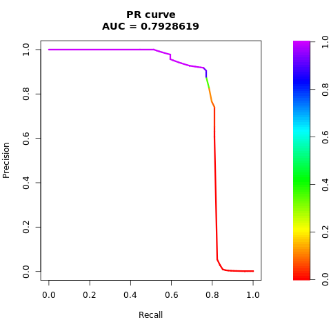
AUPRC 曲線を印刷します。
# Compute AUPRC
pr <- pr.curve(scores.class0 = fg, scores.class1 = bg, curve = TRUE)
print(pr)
AUPRC 曲線をプロットします。
# Plot AUPRC
plot(pr)
バランスの取れた (SMOTE 経由) データセット
予測を計算します。
smote_fg <- smote_preds[test_df$Class == 1]
smote_bg <- smote_preds[test_df$Class == 0]
AUC-ROC 曲線を出力します。
# Compute AUC-ROC
smote_roc <- roc.curve(scores.class0 = smote_fg, scores.class1 = smote_bg, curve = TRUE)
print(smote_roc)
AUC-ROC 曲線をプロットします。
# Plot AUC-ROC
plot(smote_roc)
AUPRC 曲線を印刷します。
# Compute AUPRC
smote_pr <- pr.curve(scores.class0 = smote_fg, scores.class1 = smote_bg, curve = TRUE)
print(smote_pr)
AUPRC 曲線をプロットします。
# Plot AUPRC
plot(smote_pr)
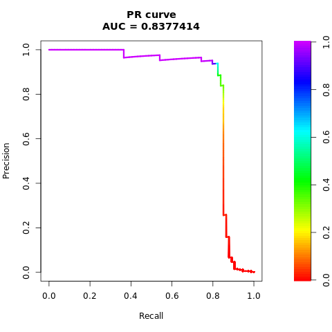
前の図では、バランスの取れたデータセットでトレーニングされたモデルが、AUC-ROC と AUPRC スコアの両方について、不均衡なデータセットでトレーニングされたモデルよりも優れていることがわかります。 この結果は、SMOTE が非常に不均衡なデータを操作する際にモデルのパフォーマンスを効果的に向上することを示唆しています。