이 자습서에서는 여러 기계 학습 모델을 학습하여 떠날 가능성이 있는 은행 고객을 예측하기 위해 가장 적합한 모델을 선택는 방법을 알아봅니다.
이 자습서에서는 다음을 수행합니다.
- 임의 포리스트 및 LightGBM 모델을 학습시킵니다.
- MLflow 프레임워크와 Microsoft Fabric의 네이티브 통합을 사용하여 학습된 기계 학습 모델, 사용된 하이퍼 매개 변수 및 평가 메트릭을 기록합니다.
- 학습되 기계 학습 모델을 등록합니다.
- 유효성 검사 데이터 세트에서 학습된 기계 학습 모델의 성능을 평가합니다.
MLflow는 추적, 모델 및 모델 레지스트리와 같은 기능을 통해 기계 학습 수명 주기를 관리하기 위한 오픈 소스 플랫폼입니다. MLflow는 기본적으로 Fabric 데이터 과학 환경과 통합되어 있습니다.
필수 조건
Microsoft Fabric 구독을 구매합니다. 또는 무료 Microsoft Fabric 평가판에 등록합니다.
Microsoft Fabric에 로그인합니다.
홈 페이지의 왼쪽 아래에 있는 환경 전환기를 사용하여 패브릭으로 전환합니다.
이 자습서의 시리즈 5부 중 3부입니다. 이 자습서를 완료하려면 먼저 다음을 완료합니다.
- 1부: Apache Spark를 사용하여 Microsoft Fabric 레이크하우스에 데이터를 수집합니다.
- 2부: Microsoft Fabric Notebook을 사용하여 데이터를 탐색하고 시각화하여 데이터에 대해 자세히 알아봅니다.
Notebooks에서 따라 하기
이 자습서에는 3-train-evaluate.ipynb Notebook이 함께 제공됩니다.
이 자습서를 위한 Notebook을 열기 위해서 데이터 과학 자습서를 위한 시스템 준비의 지침에 따라 Notebook을 작업 공간으로 가져오세요.
이 페이지에서 코드를 복사하여 붙여 넣으면 새 Notebook을 만들 수 있습니다.
코드 실행을 시작하기 전에 Notebook에 레이크하우스를 연결해야 합니다.
Important
1부와 2부에서 사용한 것과 동일한 레이크하우스를 연결합니다.
사용자 지정 라이브러리 설치
이 Notebook의 경우 imblearn을 사용하여 imbalanced-learn(%pip install로 가져옴)을 설치합니다. Imbalanced-learn은 불균형 데이터 세트를 처리할 때 사용되는 SMOTE(Synthetic Minority Oversampling Technique)용 라이브러리입니다. PySpark 커널은 %pip install 이후에 다시 시작되므로 다른 셀을 실행하기 전에 라이브러리를 설치해야 합니다.
imblearn 라이브러리를 사용하여 SMOTE에 액세스합니다. 인라인 설치 기능(예: %pip, %conda)을 사용하여 지금 설치합니다.
# Install imblearn for SMOTE using pip
%pip install imblearn
%pip install scikit-learn==1.6.1
%pip install "mlflow==2.12.2"
Important
Notebook을 다시 시작할 때마다 이 설치를 실행합니다.
Notebook에 라이브러리를 설치하는 경우 Notebook 세션 기간 동안만 사용할 수 있으며 작업 영역에서는 사용할 수 없습니다. Notebook을 다시 시작하면 라이브러리를 다시 설치해야 합니다.
자주 사용하는 라이브러리가 있고 작업 영역의 모든 Notebook에서 사용할 수 있게 하려는 경우 해당 용도로 Fabric 환경을 사용할 수 있습니다. 환경을 만들고 라이브러리를 설치한 다음, 작업 영역 관리자가 환경을 작업 영역에 기본 환경으로 연결할 수 있습니다. 환경을 작업 영역 기본값으로 설정하는 방법에 대한 자세한 내용은 작업 영역에 대한 기본 라이브러리 관리자 설정을 참조하세요.
기존 작업 영역 라이브러리 및 Spark 속성을 환경으로 마이그레이션하는 방법에 대한 자세한 내용은 작업 영역 라이브러리 및 Spark 속성을 기본 환경으로 마이그레이션을 참조하세요.
데이터 로드
기계 학습 모델을 학습하기 전에 이전 Notebook에서 만든 정리된 데이터를 읽으려면 레이크하우스에서 델타 테이블을 로드해야 합니다.
import pandas as pd
SEED = 12345
df_clean = spark.read.format("delta").load("Tables/df_clean").toPandas()
MLflow를 사용하여 모델 추적 및 로깅을 위한 실험 생성
이 섹션에서는 실험을 생성하고, 기계 학습 모델 및 학습 매개 변수를 지정하고, 메트릭을 채점하고, 기계 학습 모델을 학습시키고, 기록하고, 나중에 사용할 수 있도록 학습된 모델을 저장하는 방법을 보여 줍니다.
import mlflow
# Setup experiment name
EXPERIMENT_NAME = "bank-churn-experiment-SBM"  # MLflow experiment name
MLflow 로깅 기능을 확장하여 자동 로깅은 학습 중에 기계 학습 모델의 입력 매개 변수 및 출력 메트릭 값을 자동으로 캡처합니다. 그런 다음 이 정보는 작업 영역에 기록되며, MLflow API 또는 작업 영역의 해당 실험을 통해 액세스하고 시각화할 수 있습니다.
각 이름의 모든 실험이 기록되며 해당 매개 변수 및 성능 메트릭을 추적할 수 있습니다. 자동 로깅에 대한 자세한 내용은 Microsoft Fabric의 자동 로깅을 참조하세요.
실험 및 자동 로깅 사양 설정
mlflow.set_experiment(EXPERIMENT_NAME)
mlflow.autolog(exclusive=False)
scikit-learn 및 LightGBM 가져오기
데이터가 준비되면 이제 기계 학습 모델을 정의할 수 있습니다. 이 Notebook에서는 임의 포리스트 및 LightGBM 모델을 적용합니다.
scikit-learn 및 lightgbm을 사용하면 몇 줄의 코드로 모델을 구현할 수 있습니다.
# Import the required libraries for model training
from sklearn.model_selection import train_test_split
from lightgbm import LGBMClassifier
from sklearn.ensemble import RandomForestClassifier
from sklearn.metrics import accuracy_score, f1_score, precision_score, confusion_matrix, recall_score, roc_auc_score, classification_report
학습 및 유효성 테스트 데이터 세트 준비
train_test_split의 scikit-learn 함수를 사용하여 데이터를 학습, 유효성 검사 및 테스트 세트로 분할합니다.
y = df_clean["Exited"]
X = df_clean.drop("Exited",axis=1)
# Split the dataset to 60%, 20%, 20% for training, validation, and test datasets
# Train-Test Separation
X_train, X_test, y_train, y_test = train_test_split(X, y, test_size=0.20, random_state=SEED)
# Train-Validation Separation
X_train, X_val, y_train, y_val = train_test_split(X_train, y_train, test_size=0.25, random_state=SEED)
델타 테이블에 테스트 데이터 저장
다음 Notebook에서 사용할 수 있도록 테스트 데이터를 델타 테이블에 저장합니다.
table_name = "df_test"
# Create PySpark DataFrame from Pandas
df_test=spark.createDataFrame(X_test)
df_test.write.mode("overwrite").format("delta").save(f"Tables/{table_name}")
print(f"Spark test DataFrame saved to delta table: {table_name}")
학습 데이터에 SMOTE를 적용하여 소수 클래스에 대한 새 샘플 합성
2부의 데이터 탐색에 따르면 10,000명의 고객에 해당하는 10,000개의 데이터 요소 중 2,037명의 고객(약 20%)만이 은행을 떠난 것으로 나타났습니다. 이는 데이터 세트의 불균형이 매우 높다는 것을 나타냅니다. 불균형 분류의 문제는 모델이 의사 결정 경계를 효과적으로 학습하기에 소수 클래스의 예가 너무 적다는 것입니다. SMOTE는 소수 클래스에 대한 새 샘플을 합성하는 가장 널리 사용되는 접근 방식입니다. 여기와 여기에서 SMOTE에 대해 자세히 알아볼 수 있습니다.
팁
SMOTE는 학습 데이터 세트에만 적용되어야 합니다. 프로덕션의 상황을 나타내는 원래 데이터에서 기계 학습 모델이 어떻게 수행될지에 대한 유효한 근사치를 얻으려면 테스트 데이터 세트를 원래 불균형 배포에 남겨두어야 합니다.
from collections import Counter
from imblearn.over_sampling import SMOTE

sm = SMOTE(random_state=SEED)
X_res, y_res = sm.fit_resample(X_train, y_train)
new_train = pd.concat([X_res, y_res], axis=1)
팁
이 셀을 실행할 때 나타나는 MLflow 경고 메시지를 무시해도 됩니다.
ModuleNotFoundError 메시지가 표시되면 이 Notebook에서 imblearn 라이브러리를 설치하는 첫 번째 셀을 실행하지 못한 것입니다. Notebook을 다시 시작할 때마다 이 라이브러리를 설치해야 합니다. 돌아가서 이 Notebook의 첫 번째 셀부터 모든 셀을 다시 실행합니다.
모델 학습
- 최대 깊이 4 및 4 기능의 임의 포레스트를 사용하여 모델 학습
mlflow.sklearn.autolog(registered_model_name='rfc1_sm') # Register the trained model with autologging
rfc1_sm = RandomForestClassifier(max_depth=4, max_features=4, min_samples_split=3, random_state=1) # Pass hyperparameters
with mlflow.start_run(run_name="rfc1_sm") as run:
    rfc1_sm_run_id = run.info.run_id # Capture run_id for model prediction later
    print("run_id: {}; status: {}".format(rfc1_sm_run_id, run.info.status))
    # rfc1.fit(X_train,y_train) # Imbalanaced training data
    rfc1_sm.fit(X_res, y_res.ravel()) # Balanced training data
    rfc1_sm.score(X_val, y_val)
    y_pred = rfc1_sm.predict(X_val)
    cr_rfc1_sm = classification_report(y_val, y_pred)
    cm_rfc1_sm = confusion_matrix(y_val, y_pred)
    roc_auc_rfc1_sm = roc_auc_score(y_res, rfc1_sm.predict_proba(X_res)[:, 1])
- 최대 깊이 8 및 6 기능의 임의 포레스트를 사용하여 모델 학습
mlflow.sklearn.autolog(registered_model_name='rfc2_sm') # Register the trained model with autologging
rfc2_sm = RandomForestClassifier(max_depth=8, max_features=6, min_samples_split=3, random_state=1) # Pass hyperparameters
with mlflow.start_run(run_name="rfc2_sm") as run:
    rfc2_sm_run_id = run.info.run_id # Capture run_id for model prediction later
    print("run_id: {}; status: {}".format(rfc2_sm_run_id, run.info.status))
    # rfc2.fit(X_train,y_train) # Imbalanced training data
    rfc2_sm.fit(X_res, y_res.ravel()) # Balanced training data
    rfc2_sm.score(X_val, y_val)
    y_pred = rfc2_sm.predict(X_val)
    cr_rfc2_sm = classification_report(y_val, y_pred)
    cm_rfc2_sm = confusion_matrix(y_val, y_pred)
    roc_auc_rfc2_sm = roc_auc_score(y_res, rfc2_sm.predict_proba(X_res)[:, 1])
- LightGBM을 사용하여 모델 학습
# lgbm_model
mlflow.lightgbm.autolog(registered_model_name='lgbm_sm') # Register the trained model with autologging
lgbm_sm_model = LGBMClassifier(learning_rate = 0.07,
                        max_delta_step = 2,
                        n_estimators = 100,
                        max_depth = 10,
                        eval_metric = "logloss",
                        objective='binary',
                        random_state=42)

with mlflow.start_run(run_name="lgbm_sm") as run:
    lgbm1_sm_run_id = run.info.run_id # Capture run_id for model prediction later
    # lgbm_sm_model.fit(X_train,y_train) # Imbalanced training data
    lgbm_sm_model.fit(X_res, y_res.ravel()) # Balanced training data
    y_pred = lgbm_sm_model.predict(X_val)
    accuracy = accuracy_score(y_val, y_pred)
    cr_lgbm_sm = classification_report(y_val, y_pred)
    cm_lgbm_sm = confusion_matrix(y_val, y_pred)
    roc_auc_lgbm_sm = roc_auc_score(y_res, lgbm_sm_model.predict_proba(X_res)[:, 1])
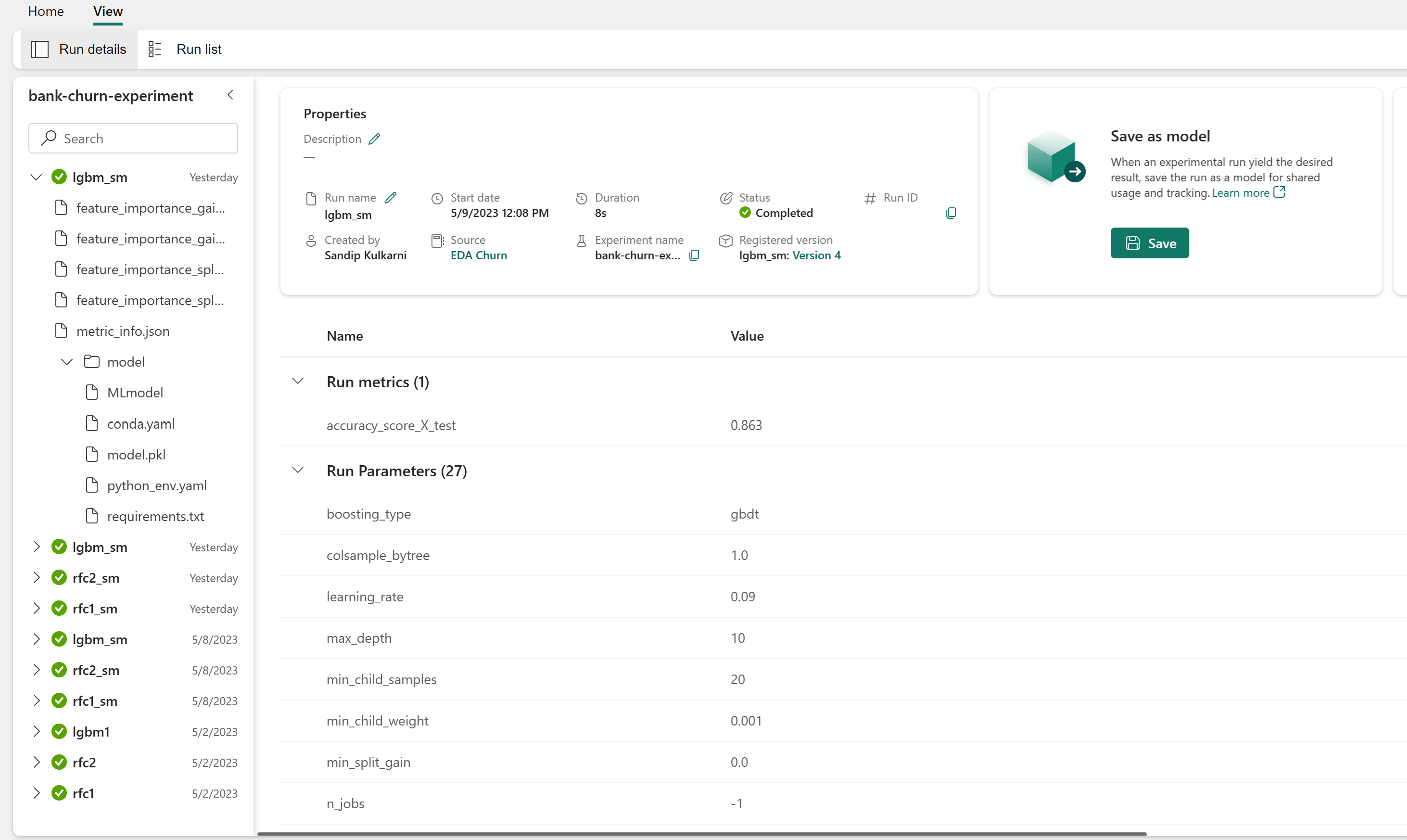
모델 성능을 추적하기 위한 실험 아티팩트
실험 실행은 작업 영역에서 찾을 수 있는 실험 아티팩트에서 자동으로 저장됩니다. 실험 설정에 사용되는 이름에 따라 이름이 지정됩니다. 학습된 모든 기계 학습 모델, 해당 실행, 성능 메트릭 및 모델 매개 변수가 기록됩니다.
실험을 보려면 다음을 수행합니다.
왼쪽 패널에서 작업 영역을 선택합니다.
오른쪽 상단에서 실험만 표시하도록 필터링하여 원하는 실험을 더 쉽게 찾을 수 있습니다.
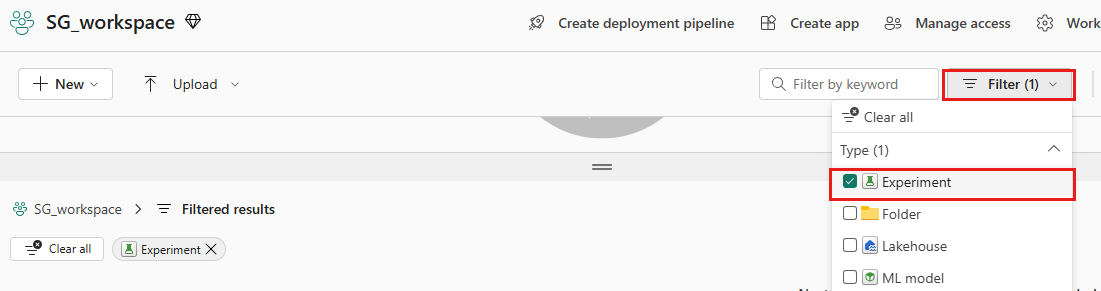
실험 이름(이 경우 bank-churn-experiment)을 찾아 선택합니다. 작업 영역에 실험이 표시되지 않으면 브라우저를 새로 고칩니다.


유효성 검사 데이터 세트에서 학습된 기계 학습 모델의 성능 평가
기계 학습 모델 학습이 완료되면 두 가지 방법으로 학습된 모델의 성능을 평가할 수 있습니다.
작업 영역에서 저장된 실험을 열고, 기계 학습 모델을 로드한 다음, 유효성 검사 데이터 세트에서 로드된 모델의 성능을 평가합니다.
# Define run_uri to fetch the model
# mlflow client: mlflow.model.url, list model
load_model_rfc1_sm = mlflow.sklearn.load_model(f"runs:/{rfc1_sm_run_id}/model")
load_model_rfc2_sm = mlflow.sklearn.load_model(f"runs:/{rfc2_sm_run_id}/model")
load_model_lgbm1_sm = mlflow.lightgbm.load_model(f"runs:/{lgbm1_sm_run_id}/model")
# Assess the performance of the loaded model on validation dataset
ypred_rfc1_sm_v1 = load_model_rfc1_sm.predict(X_val) # Random Forest with max depth of 4 and 4 features
ypred_rfc2_sm_v1 = load_model_rfc2_sm.predict(X_val) # Random Forest with max depth of 8 and 6 features
ypred_lgbm1_sm_v1 = load_model_lgbm1_sm.predict(X_val) # LightGBM
유효성 검사 데이터 세트에서 학습된 기계 학습 모델의 성능을 직접 평가합니다.
ypred_rfc1_sm_v2 = rfc1_sm.predict(X_val) # Random Forest with max depth of 4 and 4 features
ypred_rfc2_sm_v2 = rfc2_sm.predict(X_val) # Random Forest with max depth of 8 and 6 features
ypred_lgbm1_sm_v2 = lgbm_sm_model.predict(X_val) # LightGBM
선호도에 따라 두 가지 접근 방식 모두 괜찮으며 동일한 성능을 제공합니다. 이 Notebook에서는 Microsoft Fabric의 MLflow 자동 로깅 기능을 보다 잘 보여주기 위해 첫 번째 방법을 선택합니다.
혼동 행렬을 사용하여 True/False 긍정/부정
다음으로, 유효성 검사 데이터 세트를 사용하여 분류의 정확도를 평가하기 위해 혼동 행렬을 그리는 스크립트를 개발합니다. 여기에서 제공되는 사기 감지 샘플에 나와 있는 SynapseML 도구를 사용하여 혼동 행렬을 표시할 수도 있습니다.
import seaborn as sns
sns.set_theme(style="whitegrid", palette="tab10", rc = {'figure.figsize':(9,6)})
import matplotlib.pyplot as plt
import matplotlib.ticker as mticker
from matplotlib import rc, rcParams
import numpy as np
import itertools

def plot_confusion_matrix(cm, classes,
                          normalize=False,
                          title='Confusion matrix',
                          cmap=plt.cm.Blues):
    print(cm)
    plt.figure(figsize=(4,4))
    plt.rcParams.update({'font.size': 10})
    plt.imshow(cm, interpolation='nearest', cmap=cmap)
    plt.title(title)
    plt.colorbar()
    tick_marks = np.arange(len(classes))
    plt.xticks(tick_marks, classes, rotation=45, color="blue")
    plt.yticks(tick_marks, classes, color="blue")

    fmt = '.2f' if normalize else 'd'
    thresh = cm.max() / 2.
    for i, j in itertools.product(range(cm.shape[0]), range(cm.shape[1])):
        plt.text(j, i, format(cm[i, j], fmt),
                 horizontalalignment="center",
                 color="red" if cm[i, j] > thresh else "black")

    plt.tight_layout()
    plt.ylabel('True label')
    plt.xlabel('Predicted label')
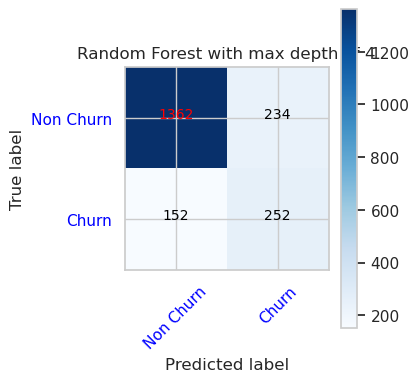
- 최대 깊이 4 및 4 기능을 갖춘 임의 포리스트 분류자의 혼동 행렬
cfm = confusion_matrix(y_val, y_pred=ypred_rfc1_sm_v1)
plot_confusion_matrix(cfm, classes=['Non Churn','Churn'],
                      title='Random Forest with max depth of 4')
tn, fp, fn, tp = cfm.ravel()
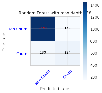
- 최대 깊이 8 및 6 기능을 갖춘 임의 포리스트 분류자의 혼동 행렬
cfm = confusion_matrix(y_val, y_pred=ypred_rfc2_sm_v1)
plot_confusion_matrix(cfm, classes=['Non Churn','Churn'],
                      title='Random Forest with max depth of 8')
tn, fp, fn, tp = cfm.ravel()
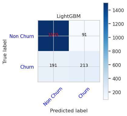
- LightGBM의 혼동 행렬
cfm = confusion_matrix(y_val, y_pred=ypred_lgbm1_sm_v1)
plot_confusion_matrix(cfm, classes=['Non Churn','Churn'],
                      title='LightGBM')
tn, fp, fn, tp = cfm.ravel()