Train regression model with Automated ML and Python (SDK v1)
APPLIES TO:  Python SDK azureml v1
In this article, you learn how to train a regression model with the Azure Machine Learning Python SDK by using Azure Machine Learning Automated ML. The regression model predicts passenger fares for taxi cabs operating in New York City (NYC). You write code with the Python SDK to configure a workspace with prepared data, train the model locally with custom parameters, and explore the results.
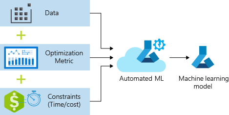
The process accepts training data and configuration settings. It automatically iterates through combinations of different feature normalization/standardization methods, models, and hyperparameter settings to arrive at the best model. The following diagram illustrates the process flow for the regression model training:
Prerequisites
An Azure subscription. You can create a free or paid account of Azure Machine Learning.
An Azure Machine Learning workspace or compute instance. To prepare these resources, see Quickstart: Get started with Azure Machine Learning.
Get the prepared sample data for the tutorial exercises by loading a notebook into your workspace:
Go to your workspace in the Azure Machine Learning studio, select Notebooks, and then select the Samples tab.
In the list of notebooks, expand the Samples > SDK v1 > tutorials > regression-automl-nyc-taxi-data node.
Select the regression-automated-ml.ipynb notebook.
To run each notebook cell as part of this tutorial, select Clone this file.
Alternate approach: If you prefer, you can run the tutorial exercises in a local environment. The tutorial is available in the Azure Machine Learning Notebooks repository on GitHub. For this approach, follow these steps to get the required packages:
Run the
pip install azureml-opendatasets azureml-widgetscommand on your local machine to get the required packages.
Download and prepare data
The Open Datasets package contains a class that represents each data source (such as NycTlcGreen) to easily filter date parameters before downloading.
The following code imports the necessary packages:
from azureml.opendatasets import NycTlcGreen
import pandas as pd
from datetime import datetime
from dateutil.relativedelta import relativedelta
The first step is to create a dataframe for the taxi data. When you work in a non-Spark environment, the Open Datasets package allows downloading only one month of data at a time with certain classes. This approach helps to avoid the MemoryError issue that can occur with large datasets.
To download the taxi data, iteratively fetch one month at a time. Before you append the next set of data to the green_taxi_df dataframe, randomly sample 2,000 records from each month, and then preview the data. This approach helps to avoid bloating the dataframe.
The following code creates the dataframe, fetches the data, and loads it into the dataframe:
green_taxi_df = pd.DataFrame([])
start = datetime.strptime("1/1/2015","%m/%d/%Y")
end = datetime.strptime("1/31/2015","%m/%d/%Y")

for sample_month in range(12):
   temp_df_green = NycTlcGreen(start + relativedelta(months=sample_month), end + relativedelta(months=sample_month)) \
      .to_pandas_dataframe()
   green_taxi_df = green_taxi_df.append(temp_df_green.sample(2000))

green_taxi_df.head(10)
The following table shows the many columns of values in the sample taxi data:
| vendorID | lpepPickupDatetime | lpepDropoffDatetime | passengerCount | tripDistance | puLocationId | doLocationId | pickupLongitude | pickupLatitude | dropoffLongitude | ... | paymentType | fareAmount | extra | mtaTax | improvementSurcharge | tipAmount | tollsAmount | ehailFee | totalAmount | tripType |
|---|---|---|---|---|---|---|---|---|---|---|---|---|---|---|---|---|---|---|---|---|
| 2 | 2015-01-30 18:38:09 | 2015-01-30 19:01:49 | 1 | 1.88 | None | None | -73.996155 | 40.690903 | -73.964287 | ... | 1 | 15.0 | 1.0 | 0.5 | 0.3 | 4.00 | 0.0 | None | 20.80 | 1.0 |
| 1 | 2015-01-17 23:21:39 | 2015-01-17 23:35:16 | 1 | 2.70 | None | None | -73.978508 | 40.687984 | -73.955116 | ... | 1 | 11.5 | 0.5 | 0.5 | 0.3 | 2.55 | 0.0 | None | 15.35 | 1.0 |
| 2 | 2015-01-16 01:38:40 | 2015-01-16 01:52:55 | 1 | 3.54 | None | None | -73.957787 | 40.721779 | -73.963005 | ... | 1 | 13.5 | 0.5 | 0.5 | 0.3 | 2.80 | 0.0 | None | 17.60 | 1.0 |
| 2 | 2015-01-04 17:09:26 | 2015-01-04 17:16:12 | 1 | 1.00 | None | None | -73.919914 | 40.826023 | -73.904839 | ... | 2 | 6.5 | 0.0 | 0.5 | 0.3 | 0.00 | 0.0 | None | 7.30 | 1.0 |
| 1 | 2015-01-14 10:10:57 | 2015-01-14 10:33:30 | 1 | 5.10 | None | None | -73.943710 | 40.825439 | -73.982964 | ... | 1 | 18.5 | 0.0 | 0.5 | 0.3 | 3.85 | 0.0 | None | 23.15 | 1.0 |
| 2 | 2015-01-19 18:10:41 | 2015-01-19 18:32:20 | 1 | 7.41 | None | None | -73.940918 | 40.839714 | -73.994339 | ... | 1 | 24.0 | 0.0 | 0.5 | 0.3 | 4.80 | 0.0 | None | 29.60 | 1.0 |
| 2 | 2015-01-01 15:44:21 | 2015-01-01 15:50:16 | 1 | 1.03 | None | None | -73.985718 | 40.685646 | -73.996773 | ... | 1 | 6.5 | 0.0 | 0.5 | 0.3 | 1.30 | 0.0 | None | 8.60 | 1.0 |
| 2 | 2015-01-12 08:01:21 | 2015-01-12 08:14:52 | 5 | 2.94 | None | None | -73.939865 | 40.789822 | -73.952957 | ... | 2 | 12.5 | 0.0 | 0.5 | 0.3 | 0.00 | 0.0 | None | 13.30 | 1.0 |
| 1 | 2015-01-16 21:54:26 | 2015-01-16 22:12:39 | 1 | 3.00 | None | None | -73.957939 | 40.721928 | -73.926247 | ... | 1 | 14.0 | 0.5 | 0.5 | 0.3 | 2.00 | 0.0 | None | 17.30 | 1.0 |
| 2 | 2015-01-06 06:34:53 | 2015-01-06 06:44:23 | 1 | 2.31 | None | None | -73.943825 | 40.810257 | -73.943062 | ... | 1 | 10.0 | 0.0 | 0.5 | 0.3 | 2.00 | 0.0 | None | 12.80 | 1.0 |
It's helpful to remove some columns that you don't need for training or other feature building. For example, you might remove the lpepPickupDatetime column because Automated ML automatically handles time-based features.
The following code removes 14 columns from the sample data:
columns_to_remove = ["lpepDropoffDatetime", "puLocationId", "doLocationId", "extra", "mtaTax",
                "improvementSurcharge", "tollsAmount", "ehailFee", "tripType", "rateCodeID",
                "storeAndFwdFlag", "paymentType", "fareAmount", "tipAmount"
               ]
for col in columns_to_remove:
   green_taxi_df.pop(col)

green_taxi_df.head(5)
Cleanse data
The next step is to cleanse the data.
The following code runs the describe() function on the new dataframe to produce summary statistics for each field:
green_taxi_df.describe()
The following table shows summary statistics for the remaining fields in the sample data:
| vendorID | passengerCount | tripDistance | pickupLongitude | pickupLatitude | dropoffLongitude | dropoffLatitude | totalAmount | |
|---|---|---|---|---|---|---|---|---|
| count | 24000.00 | 24000.00 | 24000.00 | 24000.00 | 24000.00 | 24000.00 | 24000.00 | 24000.00 |
| mean | 1.777625 | 1.373625 | 2.893981 | -73.827403 | 40.689730 | -73.819670 | 40.684436 | 14.892744 |
| std | 0.415850 | 1.046180 | 3.072343 | 2.821767 | 1.556082 | 2.901199 | 1.599776 | 12.339749 |
| min | 1.00 | 0.00 | 0.00 | -74.357101 | 0.00 | -74.342766 | 0.00 | -120.80 |
| 25% | 2.00 | 1.00 | 1.05 | -73.959175 | 40.699127 | -73.966476 | 40.699459 | 8.00 |
| 50% | 2.00 | 1.00 | 1.93 | -73.945049 | 40.746754 | -73.944221 | 40.747536 | 11.30 |
| 75% | 2.00 | 1.00 | 3.70 | -73.917089 | 40.803060 | -73.909061 | 40.791526 | 17.80 |
| max | 2.00 | 8.00 | 154.28 | 0.00 | 41.109089 | 0.00 | 40.982826 | 425.00 |
The summary statistics reveal several fields that are outliers, which are values that reduce model accuracy. To address this issue, filter the latitude/longitude (lat/long) fields so the values are within the bounds of the Manhattan area. This approach filters out longer taxi trips or trips that are outliers in respect to their relationship with other features.
Next, filter the tripDistance field for values that are greater than zero but less than 31 miles (the haversine distance between the two lat/long pairs). This technique eliminates long outlier trips that have inconsistent trip cost.
Lastly, the totalAmount field has negative values for the taxi fares, which don't make sense in the context of the model. The passengerCount field also contains bad data where the minimum value is zero.
The following code filters out these value anomalies by using query functions. The code then removes the last few columns that aren't necessary for training:
final_df = green_taxi_df.query("pickupLatitude>=40.53 and pickupLatitude<=40.88")
final_df = final_df.query("pickupLongitude>=-74.09 and pickupLongitude<=-73.72")
final_df = final_df.query("tripDistance>=0.25 and tripDistance<31")
final_df = final_df.query("passengerCount>0 and totalAmount>0")

columns_to_remove_for_training = ["pickupLongitude", "pickupLatitude", "dropoffLongitude", "dropoffLatitude"]
for col in columns_to_remove_for_training:
   final_df.pop(col)
The last step in this sequence is to call the describe() function again on the data to ensure cleansing worked as expected. You now have a prepared and cleansed set of taxi, holiday, and weather data to use for machine learning model training:
final_df.describe()
Configure workspace
Create a workspace object from the existing workspace. A Workspace is a class that accepts your Azure subscription and resource information. It also creates a cloud resource to monitor and track your model runs.
The following code calls the Workspace.from_config() function to read the config.json file and load the authentication details into an object named ws.
from azureml.core.workspace import Workspace
ws = Workspace.from_config()
The ws object is used throughout the rest of the code in this tutorial.
Split data into train and test sets
Split the data into training and test sets by using the train_test_split function in the scikit-learn library. This function segregates the data into the x (features) data set for model training and the y (values to predict) data set for testing.
The test_size parameter determines the percentage of data to allocate to testing. The random_state parameter sets a seed to the random generator, so that your train-test splits are deterministic.
The following code calls the train_test_split function to load the x and y datasets:
from sklearn.model_selection import train_test_split

x_train, x_test = train_test_split(final_df, test_size=0.2, random_state=223)
The purpose of this step is to prepare data points to test the finished model that aren't used to train the model. These points are used to measure true accuracy. A well-trained model is one that can make accurate predictions from unseen data. You now have data prepared for autotraining a machine learning model.
Automatically train model
To automatically train a model, take the following steps:
Define settings for the experiment run. Attach your training data to the configuration, and modify settings that control the training process.
Submit the experiment for model tuning. After you submit the experiment, the process iterates through different machine learning algorithms and hyperparameter settings, adhering to your defined constraints. It chooses the best-fit model by optimizing an accuracy metric.
Define training settings
Define the experiment parameter and model settings for training. View the full list of settings. Submitting the experiment with these default settings takes approximately 5-20 minutes. To decrease the run time, reduce the experiment_timeout_hours parameter.
| Property | Value in this tutorial | Description |
|---|---|---|
iteration_timeout_minutes |
10 | Time limit in minutes for each iteration. Increase this value for larger datasets that need more time for each iteration. |
experiment_timeout_hours |
0.3 | Maximum amount of time in hours that all iterations combined can take before the experiment terminates. |
enable_early_stopping |
True | Flag to enable early termination if the score isn't improving in the short term. |
primary_metric |
spearman_correlation | Metric that you want to optimize. The best-fit model is chosen based on this metric. |
featurization |
auto | The auto value allows the experiment to preprocess the input data, including handling missing data, converting text to numeric, and so on. |
verbosity |
logging.INFO | Controls the level of logging. |
n_cross_validations |
5 | Number of cross-validation splits to perform when validation data isn't specified. |
The following code submits the experiment:
import logging

automl_settings = {
   "iteration_timeout_minutes": 10,
   "experiment_timeout_hours": 0.3,
   "enable_early_stopping": True,
   "primary_metric": 'spearman_correlation',
   "featurization": 'auto',
   "verbosity": logging.INFO,
   "n_cross_validations": 5
}
The following code lets you use your defined training settings as a **kwargs parameter to an AutoMLConfig object. Additionally, you specify your training data and the type of model, which is regression in this case.
from azureml.train.automl import AutoMLConfig

automl_config = AutoMLConfig(task='regression',
                      debug_log='automated_ml_errors.log',
                      training_data=x_train,
                      label_column_name="totalAmount",
                      **automl_settings)
Note
Automated ML pre-processing steps (feature normalization, handling missing data, converting text to numeric, and so on) become part of the underlying model. When you use the model for predictions, the same pre-processing steps applied during training are applied to your input data automatically.
Train automatic regression model
Create an experiment object in your workspace. An experiment acts as a container for your individual jobs. Pass the defined automl_config object to the experiment, and set the output to True to view progress during the job.
After you start the experiment, the displayed output updates live as the experiment runs. For each iteration, you see the model type, run duration, and training accuracy. The field BEST tracks the best running training score based on your metric type:
from azureml.core.experiment import Experiment
experiment = Experiment(ws, "Tutorial-NYCTaxi")
local_run = experiment.submit(automl_config, show_output=True)
Here's the output:
Running on local machine
Parent Run ID: AutoML_1766cdf7-56cf-4b28-a340-c4aeee15b12b
Current status: DatasetFeaturization. Beginning to featurize the dataset.
Current status: DatasetEvaluation. Gathering dataset statistics.
Current status: FeaturesGeneration. Generating features for the dataset.
Current status: DatasetFeaturizationCompleted. Completed featurizing the dataset.
Current status: DatasetCrossValidationSplit. Generating individually featurized CV splits.
Current status: ModelSelection. Beginning model selection.

****************************************************************************************************
ITERATION: The iteration being evaluated.
PIPELINE: A summary description of the pipeline being evaluated.
DURATION: Time taken for the current iteration.
METRIC: The result of computing score on the fitted pipeline.
BEST: The best observed score thus far.
****************************************************************************************************

 ITERATION   PIPELINE                              DURATION     METRIC     BEST
       0   StandardScalerWrapper RandomForest          0:00:16      0.8746   0.8746
       1   MinMaxScaler RandomForest                 0:00:15      0.9468   0.9468
       2   StandardScalerWrapper ExtremeRandomTrees      0:00:09      0.9303   0.9468
       3   StandardScalerWrapper LightGBM             0:00:10      0.9424   0.9468
       4   RobustScaler DecisionTree                 0:00:09      0.9449   0.9468
       5   StandardScalerWrapper LassoLars            0:00:09      0.9440   0.9468
       6   StandardScalerWrapper LightGBM             0:00:10      0.9282   0.9468
       7   StandardScalerWrapper RandomForest          0:00:12      0.8946   0.9468
       8   StandardScalerWrapper LassoLars            0:00:16      0.9439   0.9468
       9   MinMaxScaler ExtremeRandomTrees            0:00:35      0.9199   0.9468
      10   RobustScaler ExtremeRandomTrees            0:00:19      0.9411   0.9468
      11   StandardScalerWrapper ExtremeRandomTrees      0:00:13      0.9077   0.9468
      12   StandardScalerWrapper LassoLars            0:00:15      0.9433   0.9468
      13   MinMaxScaler ExtremeRandomTrees            0:00:14      0.9186   0.9468
      14   RobustScaler RandomForest                 0:00:10      0.8810   0.9468
      15   StandardScalerWrapper LassoLars            0:00:55      0.9433   0.9468
      16   StandardScalerWrapper ExtremeRandomTrees      0:00:13      0.9026   0.9468
      17   StandardScalerWrapper RandomForest          0:00:13      0.9140   0.9468
      18   VotingEnsemble                         0:00:23      0.9471   0.9471
      19   StackEnsemble                          0:00:27      0.9463   0.9471
Explore results
Explore the results of automatic training with a Jupyter widget. The widget allows you to see a graph and table of all individual job iterations, along with training accuracy metrics and metadata. Additionally, you can filter on different accuracy metrics than your primary metric with the dropdown selector.
The following code produces a graph to explore the results:
from azureml.widgets import RunDetails
RunDetails(local_run).show()
The run details for the Jupyter widget:

The plot chart for the Jupyter widget:

Retrieve best model
The following code lets you select the best model from your iterations. The get_output function returns the best run and the fitted model for the last fit invocation. By using the overloads on the get_output function, you can retrieve the best run and fitted model for any logged metric or a particular iteration.
best_run, fitted_model = local_run.get_output()
print(best_run)
print(fitted_model)
Test best model accuracy
Use the best model to run predictions on the test data set to predict taxi fares. The predict function uses the best model and predicts the values of y, trip cost, from the x_test data set.
The following code prints the first 10 predicted cost values from the y_predict data set:
y_test = x_test.pop("totalAmount")

y_predict = fitted_model.predict(x_test)
print(y_predict[:10])
Calculate the root mean squared error of the results. Convert the y_test dataframe to a list and compare with the predicted values. The mean_squared_error function takes two arrays of values and calculates the average squared error between them. Taking the square root of the result gives an error in the same units as the y variable, cost. It indicates roughly how far the taxi fare predictions are from the actual fares.
from sklearn.metrics import mean_squared_error
from math import sqrt

y_actual = y_test.values.flatten().tolist()
rmse = sqrt(mean_squared_error(y_actual, y_predict))
rmse
Run the following code to calculate mean absolute percent error (MAPE) by using the full y_actual and y_predict data sets. This metric calculates an absolute difference between each predicted and actual value and sums all the differences. Then it expresses that sum as a percent of the total of the actual values.
sum_actuals = sum_errors = 0

for actual_val, predict_val in zip(y_actual, y_predict):
   abs_error = actual_val - predict_val
   if abs_error < 0:
      abs_error = abs_error * -1

   sum_errors = sum_errors + abs_error
   sum_actuals = sum_actuals + actual_val

mean_abs_percent_error = sum_errors / sum_actuals
print("Model MAPE:")
print(mean_abs_percent_error)
print()
print("Model Accuracy:")
print(1 - mean_abs_percent_error)
Here's the output:
Model MAPE:
0.14353867606052823

Model Accuracy:
0.8564613239394718
From the two prediction accuracy metrics, you see that the model is fairly good at predicting taxi fares from the data set's features, typically within +- $4.00, and approximately 15% error.
The traditional machine learning model development process is highly resource-intensive. It requires significant domain knowledge and time investment to run and compare the results of dozens of models. Using automated machine learning is a great way to rapidly test many different models for your scenario.
Clean up resources
If you don't plan to work on other Azure Machine Learning tutorials, complete the following steps to remove the resources you no longer need.
Stop compute
If you used a compute, you can stop the virtual machine when you aren't using it and reduce your costs:
Go to your workspace in the Azure Machine Learning studio, and select Compute.
In the list, select the compute you want to stop, and then select Stop.
When you're ready to use the compute again, you can restart the virtual machine.
Delete other resources
If you don't plan to use the resources you created in this tutorial, you can delete them and avoid incurring further charges.
Follow these steps to remove the resource group and all resources:
In the Azure portal, go to Resource groups.
In the list, select the resource group you created in this tutorial, and then select Delete resource group.
At the confirmation prompt, enter the resource group name, and then select Delete.
If you want to keep the resource group, and delete a single workspace only, follow these steps:
In the Azure portal, go to the resource group that contains the workspace you want to remove.
Select the workspace, select Properties, and then select Delete.
Next step
Maklum balas
Akan datang: Sepanjang 2024, kami akan menghentikan secara berperingkat Isu GitHub sebagai kaedah maklum balas untuk kandungan dan menggantikannya dengan sistem maklum balas baharu. Untuk mendapatkan maklumat lanjut lihat: https://aka.ms/ContentUserFeedback.
Kirim dan lihat maklum balas untuk