Quantum Computing Primer: Pure and Mixed States
This is one in a series of blog posts designed to get you up and running with Quantum Computing using Microsoft’s Q# platform. For all posts past and future, please refer to the Hitchhiker's Guide to the Quantum Computing and Q# Blog.
Introduction
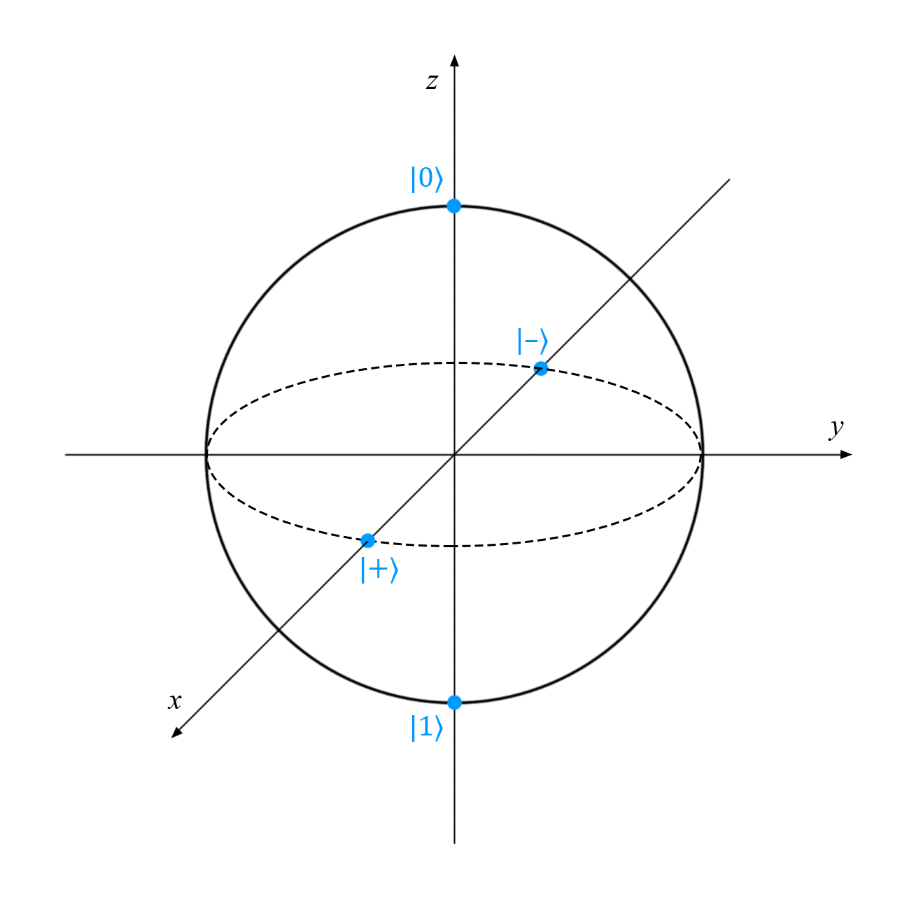
In the previous post, I introduced the Bloch Sphere as a mechanism to visualise single-qubit states. When thinking about the Bloch Sphere, we can say that all pure states exist on the surface of the sphere while mixed ones are contained within. The aim of this post is to explain what pure and mixed states actually are.
For a proper, mathematical explanation of all of this, please refer to Nielsen & Chuang’s Quantum Computation and Quantum Information, section 2.4.1: ‘Ensembles of quantum states’ or alternatively this excellent recorded lecture by Professor Leonard Susskind of Stanford.
Pure States
A pure state is any state that can be represented by a single state vector |𝜓〉. What this means in practice is that at any point in time we can say for certain (with 100% probability) that our system is in state |𝜓〉. In other words, for a pure state we have complete knowledge of the system and therefore know exactly what state it is in.
|0〉, |1〉, 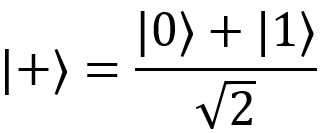 and
and  are all examples of pure states. Below we see them mapped to the surface of the Bloch Sphere:
 Mixed States
A system is in a mixed state if we have limited or no knowledge of the state that it is prepared in. There are several reasons this may be the case: for example, inconsistencies with lab equipment or entanglement with an external system that is out of our control. The upshot of this is that when we get hold of our system, we cannot be 100% sure if it is in pure state  or
or  or any number of other possible states. We therefore must describe the state of the system as a probabilistic combination of all the pure states it could possibly have been prepared in.
Let me illustrate with an example. Let’s say we have a colleague (Mary) preparing qubits for us to use in our experiment. She is trying to sabotage our results by refusing to tell us in which state she has prepared each qubit, however we know that there are only three possible options: the pure states  We must therefore describe our starting state in terms of the probability that we have been given either
  . This combination of pure states is called a mixed state.
If we know that (for example) Mary prepares  twice as often as
  or
or  , we can use these probabilities to describe the likely state of our system at the start of our experiment. If we have no knowledge at all of how Mary is choosing which state to prepare, we must assume that all states are prepared with equal probability. This is where the density matrix (AKA density operator) comes in.
The Density Operator, 𝛒
The density operator (ρ) can be used to represent the state of the system when we don’t know the starting state with certainty. It is a more general form of the state vector (used to describe pure states). The density matrix for a pure state also naturally reduces to the state vector |𝜓〉. I will work through some of the maths below for those interested.
The Maths Bit
NOTE: I am assuming basic knowledge of vector and matrix operations such as inner and outer product, orthogonality etc. For an introduction to these concepts, I’d recommend reading the Nielsen & Chuang book or the Stanford lecture series mentioned at the beginning of this post.
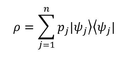
The density operator can be defined as follows:
Where:
 is the probability of the system being in state
  at the start.
- The
 element represents the outer product of the vector
  with itself, which produces a matrix (this is also known as a projection operator).
 - n is the total number of possible states the system could be in (in our example, 3).
 as you would expect (the sum of the probabilities for all possible states is equal to 1).
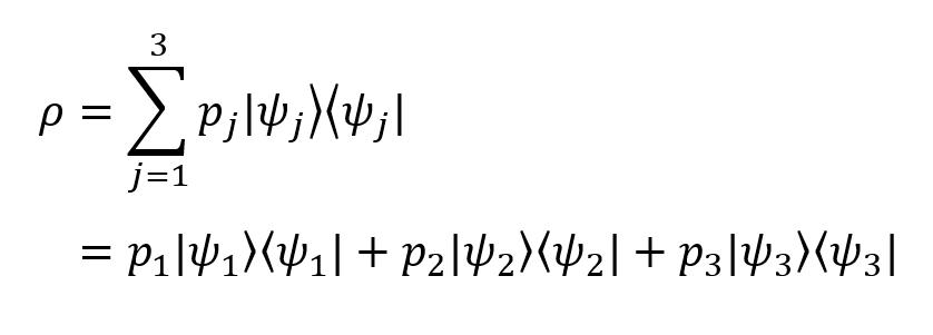
When applied to our example, the density operator expands out to look like this:
Filling in the probability values from our earlier discussion:
Which is the density matrix for our imaginary system! Not so complicated 😊
Once you’ve found the density operator, finding the probability of measuring ρ to be in some pure quantum state |ψ〉 is super-simple: it’s just 〈ψ|ρ|ψ〉.
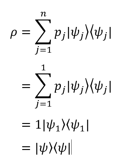
In the case that the state is a pure one (i.e. there is only one possible state the system could be in at the start), the following statement holds:
Incidentally, this has given us another definition for a pure state – any state that has a density operator ρ = |ψ〉〈ψ| a pure one (i.e. its density matrix consists of a single projector).
Now, let’s apply the density operator to our pure state vector:
As you can see, we are left with just |ψ〉.
Similarly, the probability of measuring the state to be some state |φ〉 is:
P = 〈φ |ρ|φ〉 = |〈φ|ψ〉|²
So we can see that the rules for figuring out probabilities for mixed states reduce to the rules we already know for pure states. So all the rules for mixed states reduce to those for pure states, as stated earlier 😊
