TartanAir: Conjunto de dados de simulação airSim para localização e mapeamento simultâneos (SLAM)
O SLAM (Simultaneous Localization and Mapping) é uma das capacidades mais essenciais necessária para robôs. Devido à disponibilidade universal de imagens, o Visual SLAM (V-SLAM) tornou-se num importante componente de muitos sistemas autónomos. Houve um impressionante avanço nos métodos baseados em geometria e nos métodos baseados em aprendizagem. No entanto, o desenvolvimento de métodos SLAM avançados e fiáveis para aplicações reais continua a ser um problema desafiante. Os ambientes reais estão repletos de casos difíceis, como mudança de luminosidade ou falta de iluminação, objetos dinâmicos e cenas sem textura. Este conjunto de dados tira partido da avançada tecnologia de gráficos de computador e destina-se a abranger diversos cenários com funcionalidades desafiantes em simulação.
Nota
A Microsoft fornece conjuntos de dados do Azure Open numa base "tal como está". A Microsoft não concede garantias, expressas ou implícitas, nem condições relativas à sua utilização dos conjuntos de dados. Na medida do permitido pela sua legislação local, a Microsoft declina toda a responsabilidade por quaisquer danos ou perdas, incluindo danos diretos, consequentes, especiais, indiretos, incidentais ou punitivos, resultantes da utilização dos conjuntos de dados.
Este conjunto de dados é disponibilizado de acordo com os termos originais em que a Microsoft recebeu os dados de origem. O conjunto de dados pode incluir dados obtidos junto da Microsoft.
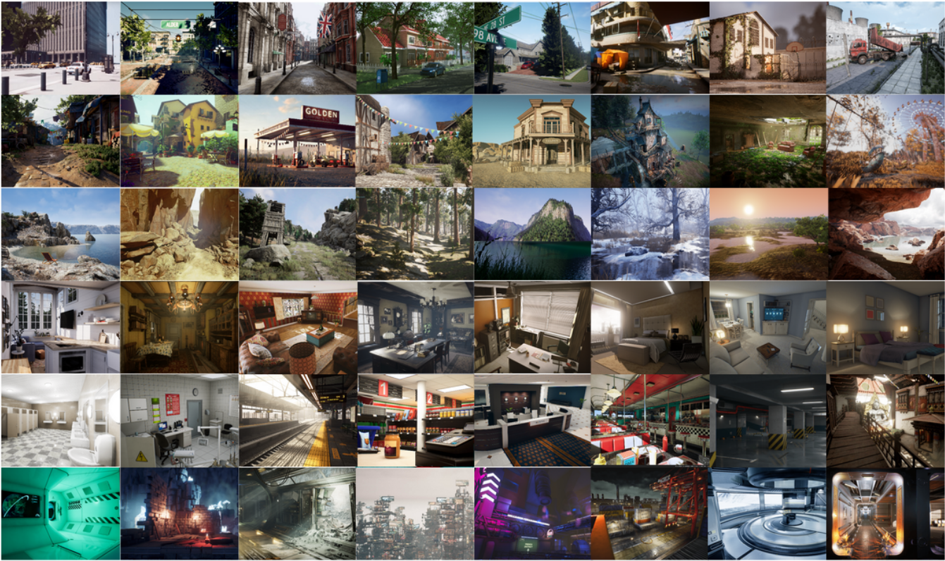
Os dados são recolhidos em ambientes de simulação foto-realistas na presença de várias condições de luz, meteorologia e objetos em movimento. Ao recolher os dados em simulação, conseguimos obter dados de sensores multimodais e etiquetas de verdade básica precisas, incluindo a imagem RGB estéreo, imagem em profundidade, segmentação, fluxo ótico e poses da câmara. Configurámos um elevado número de ambientes com vários estilos e cenas que abrangem pontos de vista desafiantes e diversos padrões de movimento, difíceis de alcançar através da utilização de plataformas de recolha de dados físicas. As quatro funcionalidades mais importantes do nosso conjunto de dados são: 1) Dados realistas de tamanho grande; 2) Etiquetas de verdade básica multimodal; 3) Diversidade de padrões de movimento; 4) Cenários Desafiantes.
Este conjunto de dados fornece cinco tipos de dados:
- Imagens estéreo: tipo de imagem (PNG)
- Ficheiro de profundidade: tipo numpy (NPY)
- Ficheiro de segmentação: tipo numpy (NPY)
- Ficheiro de fluxo ótico: tipo numpy (NPY)
- Ficheiro de pose da câmara: tipo de texto (TXT)
É recolhido de diferentes ambientes, contém centenas de trajectórias (3 TB) no total a partir de 2019.
Efeitos visuais desafiantes
Em algumas simulações, o conjunto de dados simula vários tipos de efeitos visuais desafiantes.
- Condições de fraca luminosidade. Alternar entre dia e noite. Pouca luz. Iluminações que mudam rapidamente.
- Efeitos meteorológicos. Céu limpo, chuva, neve, vento e nevoeiro.
- Mudança de estação.
Localização do armazenamento
Este conjunto de dados é armazenado na região do Azure E.U.A. Leste. A alocação de recursos de computação nos E.U.A. Leste é recomendada por questões de afinidade.
Termos de licenciamento
Este projeto é disponibilizado ao abrigo da Licença do MIT. Reveja o Ficheiro de licença para obter mais detalhes.
Informações adicionais
Veja o site oficial da TartanAir ou veja o documento de pesquisa original.
Se tiver dúvidas sobre a origem de dados, envie um e-mail para tartanair@hotmail.com. Também pode contactar os contribuidores no GitHub associado.
Citação Estão disponíveis mais detalhes técnicos em papel AirSim (FSR 2017 Conference). Cite isto como:
@article{tartanair2020arxiv,
  title =   {TartanAir: A Dataset to Push the Limits of Visual SLAM},
  author =  {Wenshan Wang, Delong Zhu, Xiangwei Wang, Yaoyu Hu, Yuheng Qiu, Chen Wang, Yafei Hu, Ashish Kapoor, Sebastian Scherer},
  journal = {arXiv preprint arXiv:2003.14338},
  year =    {2020},
  url = {https://arxiv.org/abs/2003.14338}
}
@inproceedings{airsim2017fsr,
  author = {Shital Shah and Debadeepta Dey and Chris Lovett and Ashish Kapoor},
  title = {AirSim: High-Fidelity Visual and Physical Simulation for Autonomous Vehicles},
  year = {2017},
  booktitle = {Field and Service Robotics},
  eprint = {arXiv:1705.05065},
  url = {https://arxiv.org/abs/1705.05065}
}
Acesso a dados
Utilize o seguinte exemplo de código para aceder aos dados num bloco de notas python.
Dependências
pip install numpy
pip install azure-storage-blob
pip install opencv-python
Importações e cliente de contentor
from azure.storage.blob import ContainerClient
import numpy as np
import io
import cv2
import time
import matplotlib.pyplot as plt
%matplotlib inline

# Dataset website: http://theairlab.org/tartanair-dataset/
account_url = 'https://tartanair.blob.core.windows.net/'
container_name = 'tartanair-release1'

container_client = ContainerClient(account_url=account_url,
                                 container_name=container_name,
                                 credential=None)
Ambientes e trajectórias
def get_environment_list():
    '''
    List all the environments shown in the root directory
    '''
    env_gen = container_client.walk_blobs()
    envlist = []
    for env in env_gen:
        envlist.append(env.name)
    return envlist

def get_trajectory_list(envname, easy_hard = 'Easy'):
    '''
    List all the trajectory folders, which is named as 'P0XX'
    '''
    assert(easy_hard=='Easy' or easy_hard=='Hard')
    traj_gen = container_client.walk_blobs(name_starts_with=envname + '/' + easy_hard+'/')
    trajlist = []
    for traj in traj_gen:
        trajname = traj.name
        trajname_split = trajname.split('/')
        trajname_split = [tt for tt in trajname_split if len(tt)>0]
        if trajname_split[-1][0] == 'P':
            trajlist.append(trajname)
    return trajlist

def _list_blobs_in_folder(folder_name):
    """
    List all blobs in a virtual folder in an Azure blob container
    """

    files = []
    generator = container_client.list_blobs(name_starts_with=folder_name)
    for blob in generator:
        files.append(blob.name)
    return files

def get_image_list(trajdir, left_right = 'left'):
    assert(left_right == 'left' or left_right == 'right')
    files = _list_blobs_in_folder(trajdir + '/image_' + left_right + '/')
    files = [fn for fn in files if fn.endswith('.png')]
    return files

def get_depth_list(trajdir, left_right = 'left'):
    assert(left_right == 'left' or left_right == 'right')
    files = _list_blobs_in_folder(trajdir + '/depth_' + left_right + '/')
    files = [fn for fn in files if fn.endswith('.npy')]
    return files

def get_flow_list(trajdir, ):
    files = _list_blobs_in_folder(trajdir + '/flow/')
    files = [fn for fn in files if fn.endswith('flow.npy')]
    return files

def get_flow_mask_list(trajdir, ):
    files = _list_blobs_in_folder(trajdir + '/flow/')
    files = [fn for fn in files if fn.endswith('mask.npy')]
    return files

def get_posefile(trajdir, left_right = 'left'):
    assert(left_right == 'left' or left_right == 'right')
    return trajdir + '/pose_' + left_right + '.txt'

def get_seg_list(trajdir, left_right = 'left'):
    assert(left_right == 'left' or left_right == 'right')
    files = _list_blobs_in_folder(trajdir + '/seg_' + left_right + '/')
    files = [fn for fn in files if fn.endswith('.npy')]
    return files
Listar ambientes
envlist = get_environment_list()
print('Find {} environments..'.format(len(envlist)))
print(envlist)
Listar trajectórias "fáceis" no primeiro ambiente
diff_level = 'Easy'
env_ind = 0
trajlist = get_trajectory_list(envlist[env_ind], easy_hard = diff_level)
print('Find {} trajectories in {}'.format(len(trajlist), envlist[env_ind]+diff_level))
print(trajlist)
Listar todos os ficheiros de dados numa trajetória
traj_ind = 1
traj_dir = trajlist[traj_ind]

left_img_list = get_image_list(traj_dir, left_right = 'left')
print('Find {} left images in {}'.format(len(left_img_list), traj_dir))

right_img_list = get_image_list(traj_dir, left_right = 'right')
print('Find {} right images in {}'.format(len(right_img_list), traj_dir))

left_depth_list = get_depth_list(traj_dir, left_right = 'left')
print('Find {} left depth files in {}'.format(len(left_depth_list), traj_dir))

right_depth_list = get_depth_list(traj_dir, left_right = 'right')
print('Find {} right depth files in {}'.format(len(right_depth_list), traj_dir))

left_seg_list = get_seg_list(traj_dir, left_right = 'left')
print('Find {} left segmentation files in {}'.format(len(left_seg_list), traj_dir))

right_seg_list = get_seg_list(traj_dir, left_right = 'left')
print('Find {} right segmentation files in {}'.format(len(right_seg_list), traj_dir))

flow_list = get_flow_list(traj_dir)
print('Find {} flow files in {}'.format(len(flow_list), traj_dir))

flow_mask_list = get_flow_mask_list(traj_dir)
print('Find {} flow mask files in {}'.format(len(flow_mask_list), traj_dir))

left_pose_file = get_posefile(traj_dir, left_right = 'left')
print('Left pose file: {}'.format(left_pose_file))

right_pose_file = get_posefile(traj_dir, left_right = 'right')
print('Right pose file: {}'.format(right_pose_file))
Funções de transferência de dados
def read_numpy_file(numpy_file,):
    '''
    return a numpy array given the file path
    '''
    bc = container_client.get_blob_client(blob=numpy_file)
    data = bc.download_blob()
    ee = io.BytesIO(data.content_as_bytes())
    ff = np.load(ee)
    return ff


def read_image_file(image_file,):
    '''
    return a uint8 numpy array given the file path
    '''
    bc = container_client.get_blob_client(blob=image_file)
    data = bc.download_blob()
    ee = io.BytesIO(data.content_as_bytes())
    img=cv2.imdecode(np.asarray(bytearray(ee.read()),dtype=np.uint8), cv2.IMREAD_COLOR)
    im_rgb = img[:, :, [2, 1, 0]] # BGR2RGB
    return im_rgb
Funções de visualização de dados
def depth2vis(depth, maxthresh = 50):
    depthvis = np.clip(depth,0,maxthresh)
    depthvis = depthvis/maxthresh*255
    depthvis = depthvis.astype(np.uint8)
    depthvis = np.tile(depthvis.reshape(depthvis.shape+(1,)), (1,1,3))

    return depthvis

def seg2vis(segnp):
    colors = [(205, 92, 92), (0, 255, 0), (199, 21, 133), (32, 178, 170), (233, 150, 122), (0, 0, 255), (128, 0, 0), (255, 0, 0), (255, 0, 255), (176, 196, 222), (139, 0, 139), (102, 205, 170), (128, 0, 128), (0, 255, 255), (0, 255, 255), (127, 255, 212), (222, 184, 135), (128, 128, 0), (255, 99, 71), (0, 128, 0), (218, 165, 32), (100, 149, 237), (30, 144, 255), (255, 0, 255), (112, 128, 144), (72, 61, 139), (165, 42, 42), (0, 128, 128), (255, 255, 0), (255, 182, 193), (107, 142, 35), (0, 0, 128), (135, 206, 235), (128, 0, 0), (0, 0, 255), (160, 82, 45), (0, 128, 128), (128, 128, 0), (25, 25, 112), (255, 215, 0), (154, 205, 50), (205, 133, 63), (255, 140, 0), (220, 20, 60), (255, 20, 147), (95, 158, 160), (138, 43, 226), (127, 255, 0), (123, 104, 238), (255, 160, 122), (92, 205, 92),]
    segvis = np.zeros(segnp.shape+(3,), dtype=np.uint8)

    for k in range(256):
        mask = segnp==k
        colorind = k % len(colors)
        if np.sum(mask)>0:
            segvis[mask,:] = colors[colorind]

    return segvis

def _calculate_angle_distance_from_du_dv(du, dv, flagDegree=False):
    a = np.arctan2( dv, du )

    angleShift = np.pi

    if ( True == flagDegree ):
        a = a / np.pi * 180
        angleShift = 180
        # print("Convert angle from radian to degree as demanded by the input file.")

    d = np.sqrt( du * du + dv * dv )

    return a, d, angleShift

def flow2vis(flownp, maxF=500.0, n=8, mask=None, hueMax=179, angShift=0.0):
    """
    Show a optical flow field as the KITTI dataset does.
    Some parts of this function is the transform of the original MATLAB code flow_to_color.m.
    """

    ang, mag, _ = _calculate_angle_distance_from_du_dv( flownp[:, :, 0], flownp[:, :, 1], flagDegree=False )

    # Use Hue, Saturation, Value colour model
    hsv = np.zeros( ( ang.shape[0], ang.shape[1], 3 ) , dtype=np.float32)

    am = ang < 0
    ang[am] = ang[am] + np.pi * 2

    hsv[ :, :, 0 ] = np.remainder( ( ang + angShift ) / (2*np.pi), 1 )
    hsv[ :, :, 1 ] = mag / maxF * n
    hsv[ :, :, 2 ] = (n - hsv[:, :, 1])/n

    hsv[:, :, 0] = np.clip( hsv[:, :, 0], 0, 1 ) * hueMax
    hsv[:, :, 1:3] = np.clip( hsv[:, :, 1:3], 0, 1 ) * 255
    hsv = hsv.astype(np.uint8)

    rgb = cv2.cvtColor(hsv, cv2.COLOR_HSV2RGB)

    if ( mask is not None ):
        mask = mask > 0
        rgb[mask] = np.array([0, 0 ,0], dtype=np.uint8)

    return rgb
Transferir e visualizar
data_ind = 173 # randomly select one frame (data_ind < TRAJ_LEN)

left_img = read_image_file(left_img_list[data_ind])
right_img = read_image_file(right_img_list[data_ind])

# Visualize the left and right RGB images
plt.figure(figsize=(12, 5))
plt.subplot(121)
plt.imshow(left_img)
plt.title('Left Image')
plt.subplot(122)
plt.imshow(right_img)
plt.title('Right Image')
plt.show()

# Visualize the left and right depth files
left_depth = read_numpy_file(left_depth_list[data_ind])
left_depth_vis = depth2vis(left_depth)

right_depth = read_numpy_file(right_depth_list[data_ind])
right_depth_vis = depth2vis(right_depth)

plt.figure(figsize=(12, 5))
plt.subplot(121)
plt.imshow(left_depth_vis)
plt.title('Left Depth')
plt.subplot(122)
plt.imshow(right_depth_vis)
plt.title('Right Depth')
plt.show()

# Visualize the left and right segmentation files
left_seg = read_numpy_file(left_seg_list[data_ind])
left_seg_vis = seg2vis(left_seg)

right_seg = read_numpy_file(right_seg_list[data_ind])
right_seg_vis = seg2vis(right_seg)

plt.figure(figsize=(12, 5))
plt.subplot(121)
plt.imshow(left_seg_vis)
plt.title('Left Segmentation')
plt.subplot(122)
plt.imshow(right_seg_vis)
plt.title('Right Segmentation')
plt.show()

# Visualize the flow and mask files

flow = read_numpy_file(flow_list[data_ind])
flow_vis = flow2vis(flow)

flow_mask = read_numpy_file(flow_mask_list[data_ind])
flow_vis_w_mask = flow2vis(flow, mask = flow_mask)

plt.figure(figsize=(12, 5))
plt.subplot(121)
plt.imshow(flow_vis)
plt.title('Optical Flow')
plt.subplot(122)
plt.imshow(flow_vis_w_mask)
plt.title('Optical Flow w/ Mask')
plt.show()
Passos seguintes
Veja o resto dos conjuntos de dados no catálogo Abrir Conjuntos de Dados.