Kaynak Tahmin Aracı'nı çalıştırmanın farklı yolları
Bu makalede Azure Quantum Kaynak Tahmin Aracı ile çalışmayı öğreneceksiniz. Kaynak Tahmin Aracı hem VS Code'da hem de Azure portal'da çevrimiçi olarak kullanılabilir.
Aşağıdaki tabloda Kaynak Tahmin Aracı'nı çalıştırmanın farklı yolları gösterilmektedir.
| Kullanıcı senaryosu | Platform | Öğretici |
|---|---|---|
| Q# programının kaynaklarını tahmin etme | Visual Studio Code | Sayfanın üst kısmındaki VS Code'da Q# öğesini seçin |
| Q# programının kaynaklarını tahmin etme (gelişmiş) | Visual Studio Code'da Jupyter Notebook | Sayfanın üst kısmındaki Jupyter Notebook Q# seçeneğini belirleyin |
| Qiskit programının kaynaklarını tahmin eder | Azure Quantum portalı | Sayfanın üst kısmındaki Azure portal Qiskit'i seçin |
| QIR programının kaynaklarını tahmin edin | Azure Quantum portalı | QIR gönderme |
| FCIDUMP dosyalarını bağımsız değişken parametreleri olarak kullanma (gelişmiş) | Visual Studio Code | Kuantum kimyası sorunu gönderme |
Not
Microsoft Quantum Geliştirme Seti (Klasik QDK) artık 30 Haziran 2024'e kadar desteklenmeyecektir. Mevcut bir QDK geliştiricisiyseniz kuantum çözümleri geliştirmeye devam etmek için yeni Azure Quantum Development Kit'e (Modern QDK) geçmenizi öneririz. Daha fazla bilgi için bkz . Q# kodunuzu Modern QDK'ye geçirme.
VS Code önkoşulları
- Visual Studio Code'nin en son sürümü veya Web'de VS Code'un açılması.
- Azure Quantum Development Kit uzantısının en son sürümü. Yükleme ayrıntıları için bkz . VS Code'da Modern QDK'yi yükleme.
İpucu
Yerel Kaynak Tahmin Aracı'nı çalıştırmak için bir Azure hesabınız olması gerekmez.
Yeni bir Q# dosyası İçerik Oluşturucu
- yeni bir dosya oluşturmak için Visual Studio Code açın ve Dosya > Yeni Metin Dosyası'na tıklayın.
- Dosyayı
ShorRE.qsolarak kaydedin. Bu dosya, programınız için Q# kodunu içerir.
Kuantum algoritmasını İçerik Oluşturucu
Aşağıdaki kodu dosyaya ShorRE.qs kopyalayın:
namespace Shors {
    open Microsoft.Quantum.Arrays;
    open Microsoft.Quantum.Canon;
    open Microsoft.Quantum.Convert;
    open Microsoft.Quantum.Diagnostics;
    open Microsoft.Quantum.Intrinsic;
    open Microsoft.Quantum.Math;
    open Microsoft.Quantum.Measurement;
    open Microsoft.Quantum.Unstable.Arithmetic;
    open Microsoft.Quantum.ResourceEstimation;

    @EntryPoint()
    operation RunProgram() : Unit {
        let bitsize = 31;

        // When chooseing parameters for `EstimateFrequency`, make sure that
        // generator and modules are not co-prime
        let _ = EstimateFrequency(11, 2^bitsize - 1, bitsize);
    }

    // In this sample we concentrate on costing the `EstimateFrequency`
    // operation, which is the core quantum operation in Shors algorithm, and
    // we omit the classical pre- and post-processing.

    /// # Summary
    /// Estimates the frequency of a generator
    /// in the residue ring Z mod `modulus`.
    ///
    /// # Input
    /// ## generator
    /// The unsigned integer multiplicative order (period)
    /// of which is being estimated. Must be co-prime to `modulus`.
    /// ## modulus
    /// The modulus which defines the residue ring Z mod `modulus`
    /// in which the multiplicative order of `generator` is being estimated.
    /// ## bitsize
    /// Number of bits needed to represent the modulus.
    ///
    /// # Output
    /// The numerator k of dyadic fraction k/2^bitsPrecision
    /// approximating s/r.
    operation EstimateFrequency(
        generator : Int,
        modulus : Int,
        bitsize : Int
    )
    : Int {
        mutable frequencyEstimate = 0;
        let bitsPrecision =  2 * bitsize + 1;

        // Allocate qubits for the superposition of eigenstates of
        // the oracle that is used in period finding.
        use eigenstateRegister = Qubit[bitsize];

        // Initialize eigenstateRegister to 1, which is a superposition of
        // the eigenstates we are estimating the phases of.
        // We first interpret the register as encoding an unsigned integer
        // in little endian encoding.
        ApplyXorInPlace(1, eigenstateRegister);
        let oracle = ApplyOrderFindingOracle(generator, modulus, _, _);

        // Use phase estimation with a semiclassical Fourier transform to
        // estimate the frequency.
        use c = Qubit();
        for idx in bitsPrecision - 1..-1..0 {
            within {
                H(c);
            } apply {
                // `BeginEstimateCaching` and `EndEstimateCaching` are the operations
                // exposed by Azure Quantum Resource Estimator. These will instruct
                // resource counting such that the if-block will be executed
                // only once, its resources will be cached, and appended in
                // every other iteration.
                if BeginEstimateCaching("ControlledOracle", SingleVariant()) {
                    Controlled oracle([c], (1 <<< idx, eigenstateRegister));
                    EndEstimateCaching();
                }
                R1Frac(frequencyEstimate, bitsPrecision - 1 - idx, c);
            }
            if MResetZ(c) == One {
                set frequencyEstimate += 1 <<< (bitsPrecision - 1 - idx);
            }
        }

        // Return all the qubits used for oracles eigenstate back to 0 state
        // using Microsoft.Quantum.Intrinsic.ResetAll.
        ResetAll(eigenstateRegister);

        return frequencyEstimate;
    }

    /// # Summary
    /// Interprets `target` as encoding unsigned little-endian integer k
    /// and performs transformation |k⟩ ↦ |gᵖ⋅k mod N ⟩ where
    /// p is `power`, g is `generator` and N is `modulus`.
    ///
    /// # Input
    /// ## generator
    /// The unsigned integer multiplicative order ( period )
    /// of which is being estimated. Must be co-prime to `modulus`.
    /// ## modulus
    /// The modulus which defines the residue ring Z mod `modulus`
    /// in which the multiplicative order of `generator` is being estimated.
    /// ## power
    /// Power of `generator` by which `target` is multiplied.
    /// ## target
    /// Register interpreted as little endian encoded which is multiplied by
    /// given power of the generator. The multiplication is performed modulo
    /// `modulus`.
    internal operation ApplyOrderFindingOracle(
        generator : Int, modulus : Int, power : Int, target : Qubit[]
    )
    : Unit
    is Adj + Ctl {
        // The oracle we use for order finding implements |x⟩ ↦ |x⋅a mod N⟩. We
        // also use `ExpModI` to compute a by which x must be multiplied. Also
        // note that we interpret target as unsigned integer in little-endian
        // encoding.
        ModularMultiplyByConstant(modulus,
                                    ExpModI(generator, power, modulus),
                                    target);
    }

    /// # Summary
    /// Performs modular in-place multiplication by a classical constant.
    ///
    /// # Description
    /// Given the classical constants `c` and `modulus`, and an input
    /// quantum register  |𝑦⟩, this operation
    /// computes `(c*x) % modulus` into |𝑦⟩.
    ///
    /// # Input
    /// ## modulus
    /// Modulus to use for modular multiplication
    /// ## c
    /// Constant by which to multiply |𝑦⟩
    /// ## y
    /// Quantum register of target
    internal operation ModularMultiplyByConstant(modulus : Int, c : Int, y : Qubit[])
    : Unit is Adj + Ctl {
        use qs = Qubit[Length(y)];
        for (idx, yq) in Enumerated(y) {
            let shiftedC = (c <<< idx) % modulus;
            Controlled ModularAddConstant([yq], (modulus, shiftedC, qs));
        }
        ApplyToEachCA(SWAP, Zipped(y, qs));
        let invC = InverseModI(c, modulus);
        for (idx, yq) in Enumerated(y) {
            let shiftedC = (invC <<< idx) % modulus;
            Controlled ModularAddConstant([yq], (modulus, modulus - shiftedC, qs));
        }
    }

    /// # Summary
    /// Performs modular in-place addition of a classical constant into a
    /// quantum register.
    ///
    /// # Description
    /// Given the classical constants `c` and `modulus`, and an input
    /// quantum register  |𝑦⟩, this operation
    /// computes `(x+c) % modulus` into |𝑦⟩.
    ///
    /// # Input
    /// ## modulus
    /// Modulus to use for modular addition
    /// ## c
    /// Constant to add to |𝑦⟩
    /// ## y
    /// Quantum register of target
    internal operation ModularAddConstant(modulus : Int, c : Int, y : Qubit[])
    : Unit is Adj + Ctl {
        body (...) {
            Controlled ModularAddConstant([], (modulus, c, y));
        }
        controlled (ctrls, ...) {
            // We apply a custom strategy to control this operation instead of
            // letting the compiler create the controlled variant for us in which
            // the `Controlled` functor would be distributed over each operation
            // in the body.
            //
            // Here we can use some scratch memory to save ensure that at most one
            // control qubit is used for costly operations such as `AddConstant`
            // and `CompareGreaterThenOrEqualConstant`.
            if Length(ctrls) >= 2 {
                use control = Qubit();
                within {
                    Controlled X(ctrls, control);
                } apply {
                    Controlled ModularAddConstant([control], (modulus, c, y));
                }
            } else {
                use carry = Qubit();
                Controlled AddConstant(ctrls, (c, y + [carry]));
                Controlled Adjoint AddConstant(ctrls, (modulus, y + [carry]));
                Controlled AddConstant([carry], (modulus, y));
                Controlled CompareGreaterThanOrEqualConstant(ctrls, (c, y, carry));
            }
        }
    }

    /// # Summary
    /// Performs in-place addition of a constant into a quantum register.
    ///
    /// # Description
    /// Given a non-empty quantum register |𝑦⟩ of length 𝑛+1 and a positive
    /// constant 𝑐 < 2ⁿ, computes |𝑦 + c⟩ into |𝑦⟩.
    ///
    /// # Input
    /// ## c
    /// Constant number to add to |𝑦⟩.
    /// ## y
    /// Quantum register of second summand and target; must not be empty.
    internal operation AddConstant(c : Int, y : Qubit[]) : Unit is Adj + Ctl {
        // We are using this version instead of the library version that is based
        // on Fourier angles to show an advantage of sparse simulation in this sample.

        let n = Length(y);
        Fact(n > 0, "Bit width must be at least 1");

        Fact(c >= 0, "constant must not be negative");
        Fact(c < 2 ^ n, $"constant must be smaller than {2L ^ n}");

        if c != 0 {
            // If c has j trailing zeroes than the j least significant bits
            // of y won't be affected by the addition and can therefore be
            // ignored by applying the addition only to the other qubits and
            // shifting c accordingly.
            let j = NTrailingZeroes(c);
            use x = Qubit[n - j];
            within {
                ApplyXorInPlace(c >>> j, x);
            } apply {
                IncByLE(x, y[j...]);
            }
        }
    }

    /// # Summary
    /// Performs greater-than-or-equals comparison to a constant.
    ///
    /// # Description
    /// Toggles output qubit `target` if and only if input register `x`
    /// is greater than or equal to `c`.
    ///
    /// # Input
    /// ## c
    /// Constant value for comparison.
    /// ## x
    /// Quantum register to compare against.
    /// ## target
    /// Target qubit for comparison result.
    ///
    /// # Reference
    /// This construction is described in [Lemma 3, arXiv:2201.10200]
    internal operation CompareGreaterThanOrEqualConstant(c : Int, x : Qubit[], target : Qubit)
    : Unit is Adj+Ctl {
        let bitWidth = Length(x);

        if c == 0 {
            X(target);
        } elif c >= 2 ^ bitWidth {
            // do nothing
        } elif c == 2 ^ (bitWidth - 1) {
            ApplyLowTCNOT(Tail(x), target);
        } else {
            // normalize constant
            let l = NTrailingZeroes(c);

            let cNormalized = c >>> l;
            let xNormalized = x[l...];
            let bitWidthNormalized = Length(xNormalized);
            let gates = Rest(IntAsBoolArray(cNormalized, bitWidthNormalized));

            use qs = Qubit[bitWidthNormalized - 1];
            let cs1 = [Head(xNormalized)] + Most(qs);
            let cs2 = Rest(xNormalized);

            within {
                for i in IndexRange(gates) {
                    (gates[i] ? ApplyAnd | ApplyOr)(cs1[i], cs2[i], qs[i]);
                }
            } apply {
                ApplyLowTCNOT(Tail(qs), target);
            }
        }
    }

    /// # Summary
    /// Internal operation used in the implementation of GreaterThanOrEqualConstant.
    internal operation ApplyOr(control1 : Qubit, control2 : Qubit, target : Qubit) : Unit is Adj {
        within {
            ApplyToEachA(X, [control1, control2]);
        } apply {
            ApplyAnd(control1, control2, target);
            X(target);
        }
    }

    internal operation ApplyAnd(control1 : Qubit, control2 : Qubit, target : Qubit)
    : Unit is Adj {
        body (...) {
            CCNOT(control1, control2, target);
        }
        adjoint (...) {
            H(target);
            if (M(target) == One) {
                X(target);
                CZ(control1, control2);
            }
        }
    }


    /// # Summary
    /// Returns the number of trailing zeroes of a number
    ///
    /// ## Example
    /// ```qsharp
    /// let zeroes = NTrailingZeroes(21); // = NTrailingZeroes(0b1101) = 0
    /// let zeroes = NTrailingZeroes(20); // = NTrailingZeroes(0b1100) = 2
    /// ```
    internal function NTrailingZeroes(number : Int) : Int {
        mutable nZeroes = 0;
        mutable copy = number;
        while (copy % 2 == 0) {
            set nZeroes += 1;
            set copy /= 2;
        }
        return nZeroes;
    }

    /// # Summary
    /// An implementation for `CNOT` that when controlled using a single control uses
    /// a helper qubit and uses `ApplyAnd` to reduce the T-count to 4 instead of 7.
    internal operation ApplyLowTCNOT(a : Qubit, b : Qubit) : Unit is Adj+Ctl {
        body (...) {
            CNOT(a, b);
        }

        adjoint self;

        controlled (ctls, ...) {
            // In this application this operation is used in a way that
            // it is controlled by at most one qubit.
            Fact(Length(ctls) <= 1, "At most one control line allowed");

            if IsEmpty(ctls) {
                CNOT(a, b);
            } else {
                use q = Qubit();
                within {
                    ApplyAnd(Head(ctls), a, q);
                } apply {
                    CNOT(q, b);
                }
            }
        }

        controlled adjoint self;
    }
}
Kaynak Tahmin Aracı'nı çalıştırma
Kaynak Tahmin Aracı, dördü kapı tabanlı yönerge kümelerine ve ikisi de Majorana yönerge kümesine sahip olmak üzere önceden tanımlanmış altı kubit parametresi sunar. Ayrıca iki kuantum hata düzeltme kodusurface_code ve floquet_codesunar.
Bu örnekte, qubit parametresini ve kuantum hata düzeltme kodunu kullanarak qubit_gate_us_e3 Kaynak Tahmin Aracı'nı surface_code çalıştırırsınız.
Görünüm -> Komut Paleti'ni seçin ve Q#: Kaynak Tahminlerini Hesapla seçeneğinin görüntülenmesi gereken "kaynak" yazın. Aşağıdaki
@EntryPoint()komut listesinden Tahmin'e de tıklayabilirsiniz. Kaynak Tahmin Aracı penceresini açmak için bu seçeneği belirleyin.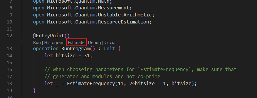
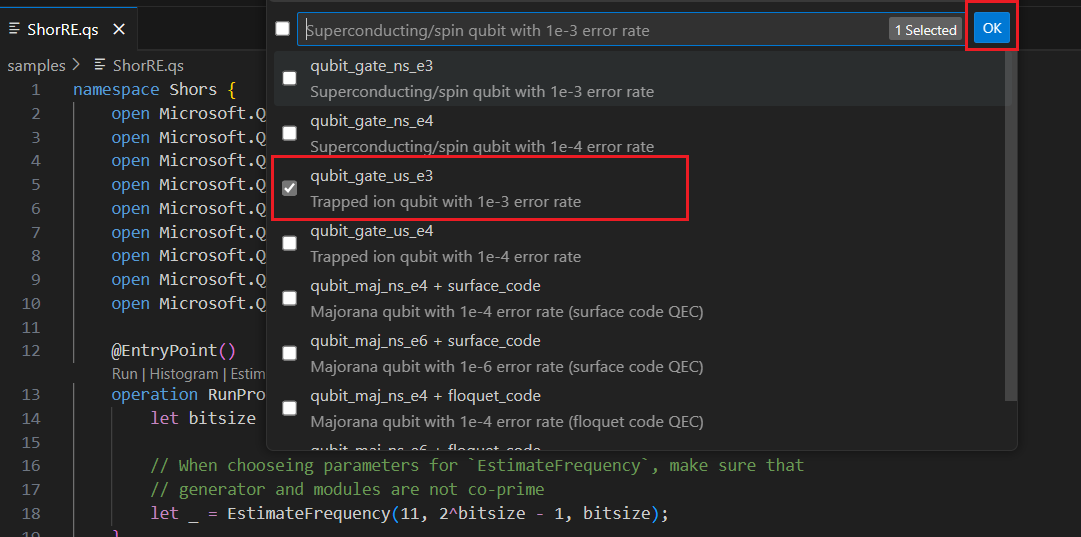
Kaynaklarını tahmin etmek için bir veya daha fazla Qubit parametresi + Hata Düzeltmesi kod türü seçebilirsiniz. Bu örnekte qubit_gate_us_e3 seçin ve Tamam'a tıklayın.
Hata bütçesini belirtin veya varsayılan 0,001 değerini kabul edin. Bu örnekte varsayılan değeri bırakın ve Enter tuşuna basın.
Bu örnekte ShorRE adlı dosya adına göre varsayılan sonuç adını kabul etmek için Enter tuşuna basın.
Sonuçları görüntüleme
Kaynak Tahmin Aracı aynı algoritma için birden çok tahmin sağlar ve her biri kubit sayısı ile çalışma zamanı arasındaki dengeleri gösterir. Çalışma zamanı ile sistem ölçeği arasındaki dengeyi anlamak, kaynak tahmininin en önemli yönlerinden biridir.
Kaynak tahmininin sonucu Q# Tahmini penceresinde görüntülenir.
Sonuçlar sekmesinde kaynak tahmininin özeti görüntülenir. Görüntülemek istediğiniz sütunları seçmek için ilk satırın yanındaki simgeye tıklayın. Çalıştırma adı, tahmin türü, kubit türü, qec şeması, hata bütçesi, mantıksal kubitler, mantıksal derinlik, kod uzaklığı, T durumları, T fabrikaları, T fabrika kesri, çalışma zamanı, rQOPS ve fiziksel kubitler arasından seçim yapabilirsiniz.
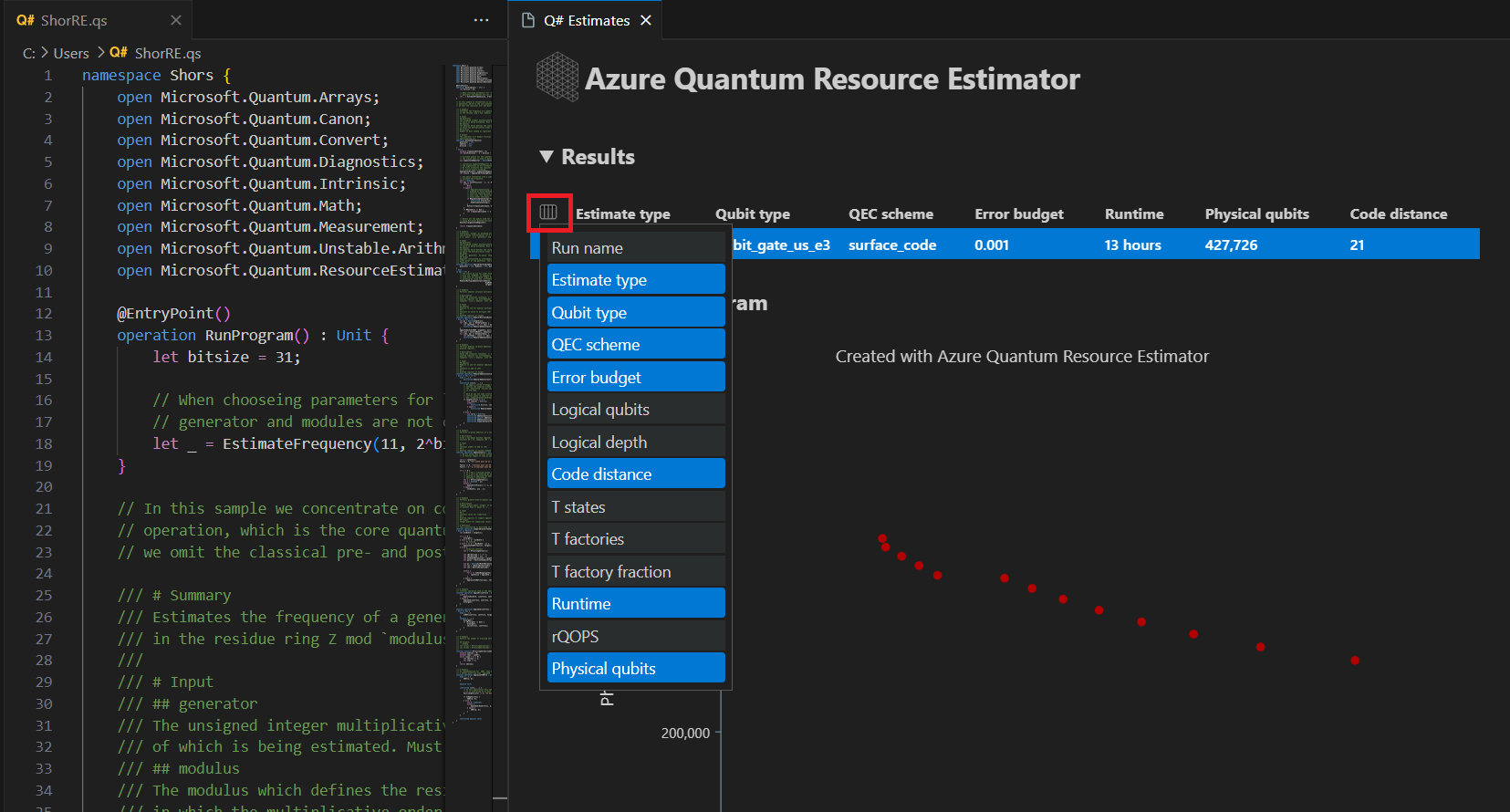
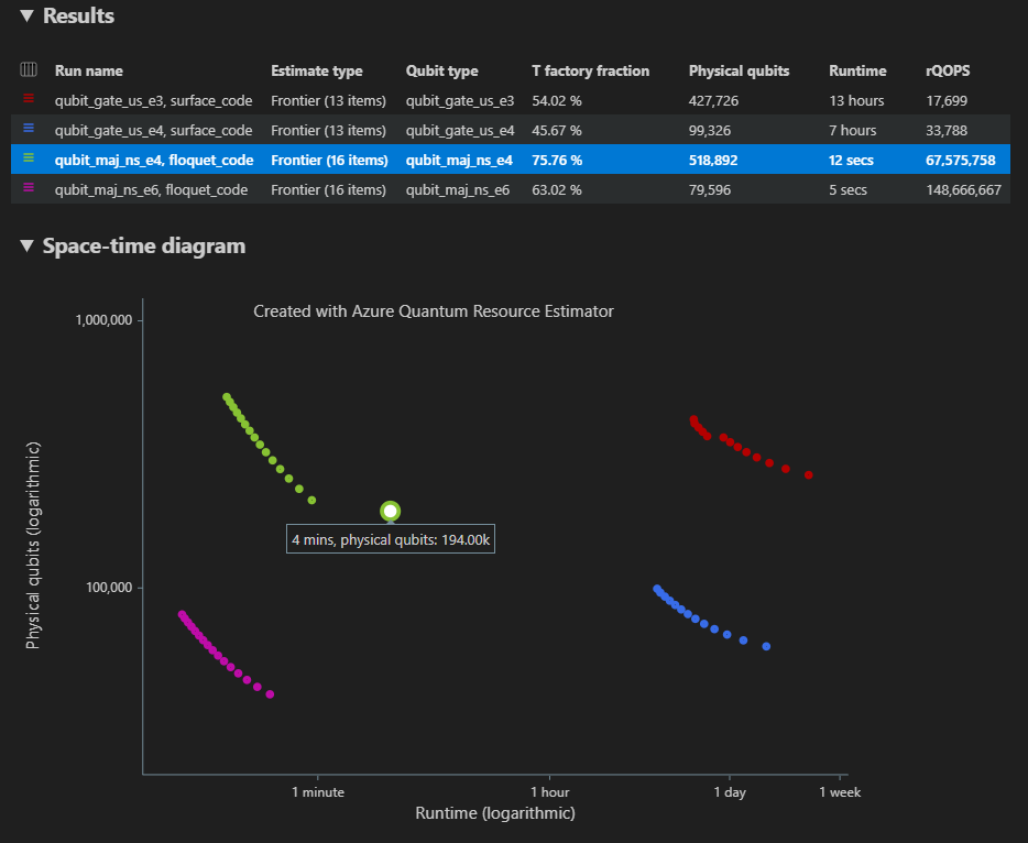
Sonuçlar tablosunun Tahmin türü sütununda algoritmanız için en uygun {kubit sayısı, çalışma zamanı} birleşimi sayısını görebilirsiniz. Bu birleşimler uzay-zaman diyagramında görülebilir.
Uzay-zaman diyagramı, fiziksel kubit sayısı ile algoritmanın çalışma zamanı arasındaki dengeleri gösterir. Bu durumda Kaynak Tahmin Aracı, binlerce olası kombinasyondan 13 farklı en uygun kombinasyon bulur. Bu noktada kaynak tahmininin ayrıntılarını görmek için her {kubit sayısı, çalışma zamanı} noktasının üzerine gelebilirsiniz.
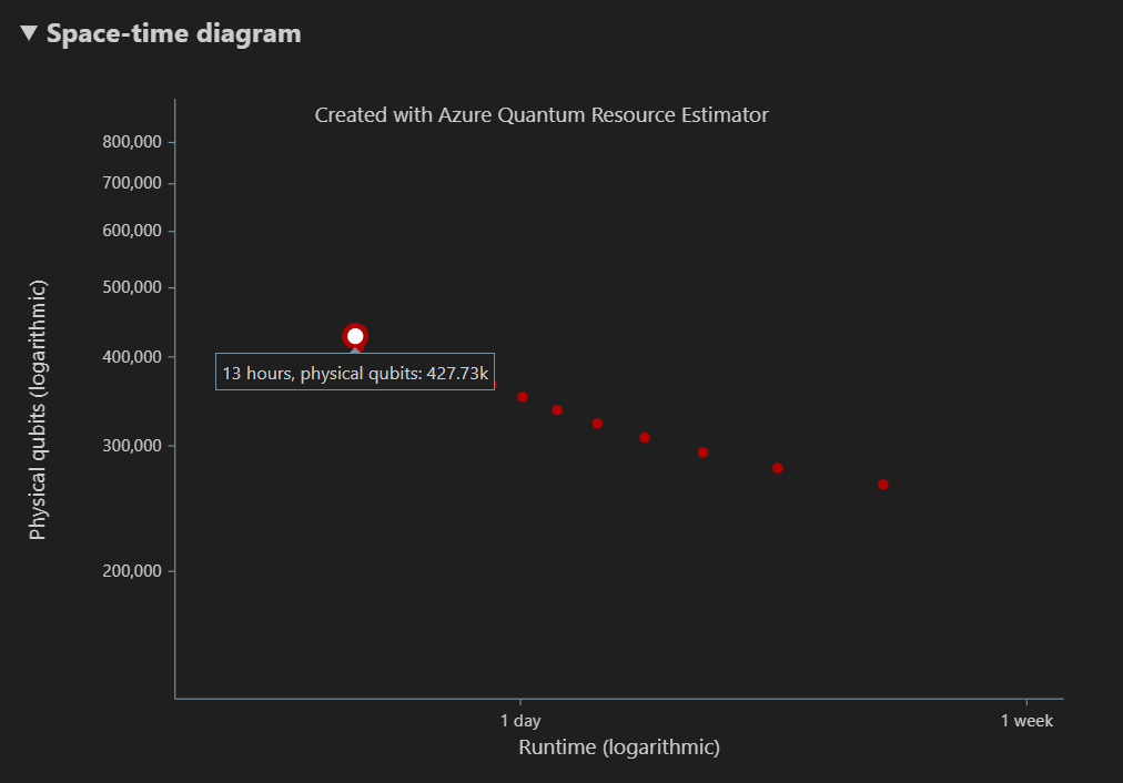
Daha fazla bilgi için bkz . Uzay-zaman diyagramı.
Not
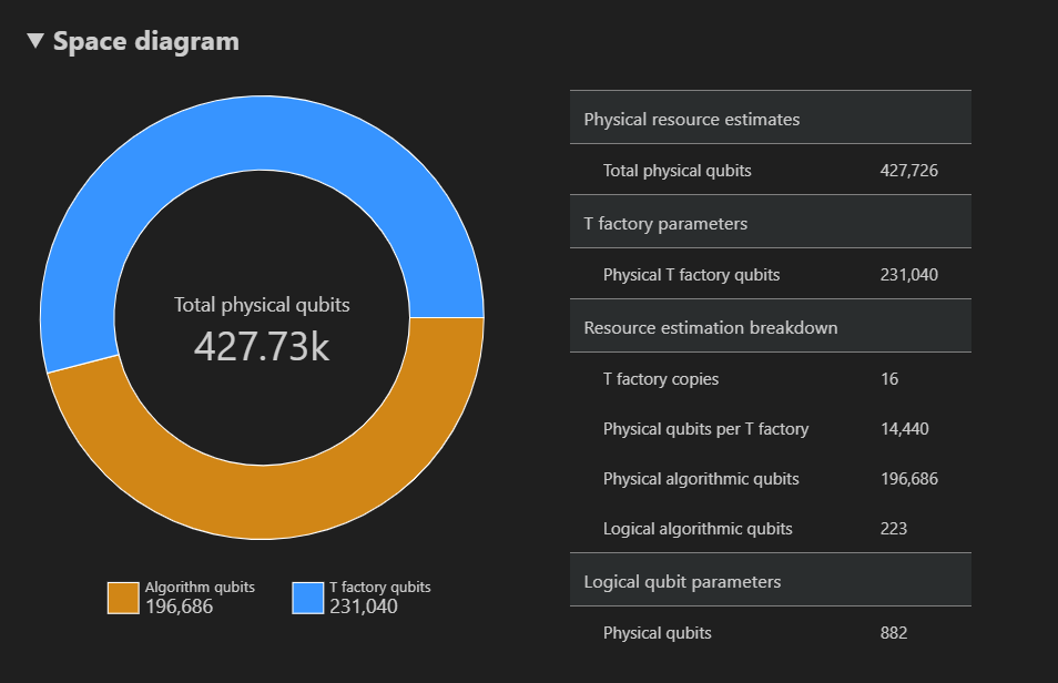
Alan diyagramını ve bu noktaya karşılık gelen kaynak tahmininin ayrıntılarını görmek için boşluk zamanı diyagramının bir noktasına ({kubit sayısı, çalışma zamanı} çifti) tıklamanız gerekir.
Alan diyagramı, algoritma için kullanılan fiziksel kubitlerin ve bir {kubit sayısı, çalışma zamanı} çiftine karşılık gelen T fabrikalarının dağılımını gösterir. Örneğin, uzay zamanı diyagramında en soldaki noktayı seçerseniz, algoritmayı çalıştırmak için gereken fiziksel kubitlerin sayısı 427726 196686 algoritma kubitleri ve 231040'ı T factory kubitleridir.
Son olarak, Kaynak Tahminleri sekmesinde {kubit sayısı, çalışma zamanı} çiftine karşılık gelen Kaynak Tahmin Aracı'nın çıktı verilerinin tam listesi görüntülenir. Daha fazla bilgi içeren grupları daraltarak maliyet ayrıntılarını inceleyebilirsiniz. Örneğin, uzay-zaman diyagramında en soldaki noktayı seçin ve Mantıksal kubit parametreleri grubunu daraltın.
Mantıksal kubit parametresi Değer QEC şeması surface_code Kod uzaklığı 21 Fiziksel kubitler 882 Mantıksal döngü süresi 13 miliseks Mantıksal kubit hata oranı 3.00E-13 Ön düzenlemeyi geçme 0.03 Hata düzeltme eşiği 0.01 Mantıksal döngü süresi formülü (4 * twoQubitGateTime+ 2 *oneQubitMeasurementTime) *codeDistanceFiziksel kubit formülü 2 * codeDistance*codeDistanceİpucu
Rapor verilerinin her çıkışının açıklamasını görüntülemek için Ayrıntılı satırları göster'e tıklayın.
Daha fazla bilgi için bkz. Kaynak Tahmin Aracı'nın tüm rapor verileri.
target Parametreleri değiştirme
Diğer kubit türünü, hata düzeltme kodunu ve hata bütçesini kullanarak aynı Q# programının maliyetini tahmin edebilirsiniz. Görünüm -> Komut Paleti'ni seçerek Kaynak Tahmin Aracı penceresini açın ve yazınQ#: Calculate Resource Estimates.
Majorana tabanlı kubit parametresi qubit_maj_ns_e6gibi başka bir yapılandırma seçin. Varsayılan hata bütçe değerini kabul edin veya yenisini girin ve Enter tuşuna basın. Kaynak Tahmin Aracı, tahmini yeni target parametrelerle yeniden çalıştırır.
Daha fazla bilgi için bkz. Kaynak Tahmin Aracı için hedef parametreler .
Parametrelerin birden çok yapılandırmasını çalıştırma
Azure Quantum Kaynak Tahmin Aracı birden çok parametre yapılandırması target çalıştırabilir ve kaynak tahmin sonuçlarını karşılaştırabilir.
Görünüm -> Komut Paleti'ne tıklayın veya Ctrl+Shift+P tuşlarına basın ve yazın
Q#: Calculate Resource Estimates.qubit_gate_us_e3, qubit_gate_us_e4, qubit_maj_ns_e4 + floquet_code ve qubit_maj_ns_e6 + floquet_code'ı seçin ve Tamam'a tıklayın.
Varsayılan hata bütçe değeri 0,001'i kabul edin ve Enter tuşuna basın.
Bu örnekte ShorRE.qs giriş dosyasını kabul etmek için Enter tuşuna basın.
Parametrelerin birden çok yapılandırması söz konusu olduğunda sonuçlar Sonuçlar sekmesinde farklı satırlarda görüntülenir.
Space-time diyagramı, parametrelerin tüm yapılandırmalarının sonuçlarını gösterir. Sonuç tablosunun ilk sütunu, parametrelerin her yapılandırması için göstergeyi görüntüler. Bu noktada kaynak tahmininin ayrıntılarını görmek için her noktanın üzerine gelebilirsiniz.
Karşılık gelen alan diyagramını ve rapor verilerini getirmek için uzay-zaman diyagramının {kubit sayısı, çalışma zamanı} noktasına tıklayın.
VS Code'da Jupyter Notebook önkoşulları
Python ve Pip'in yüklü olduğu bir Python ortamı.
Visual Studio Code'nin en son sürümü veya Web'de VS Code'u açın.
Azure Quantum Geliştirme Seti, Python ve Jupyter uzantılarının yüklü olduğu VS Code.
En son Azure Quantum
qsharpveqsharp-widgetspaketleri.python -m pip install --upgrade qsharp qsharp-widgets
İpucu
Yerel Kaynak Tahmin Aracı'nı çalıştırmak için bir Azure hesabınız olması gerekmez.
Kuantum algoritmasını İçerik Oluşturucu
VS Code'da Komut paleti Görüntüle'yi > seçin ve İçerik Oluşturucu: Yeni Jupyter Notebook'ı seçin.
Sağ üst kısımda VS Code, not defteri için seçilen Python sürümünü ve sanal Python ortamını algılar ve görüntüler. Birden çok Python ortamınız varsa, sağ üstteki çekirdek seçiciyi kullanarak bir çekirdek seçmeniz gerekebilir. Ortam algılanmadıysa kurulum bilgileri için VS Code'da Jupyter Notebooks bölümüne bakın.
Not defterinin ilk hücresinde paketi içeri aktarın
qsharp.import qsharpYeni bir hücre ekleyin ve aşağıdaki kodu kopyalayın.
%%qsharp
open Microsoft.Quantum.Arrays;
open Microsoft.Quantum.Canon;
open Microsoft.Quantum.Convert;
open Microsoft.Quantum.Diagnostics;
open Microsoft.Quantum.Intrinsic;
open Microsoft.Quantum.Math;
open Microsoft.Quantum.Measurement;
open Microsoft.Quantum.Unstable.Arithmetic;
open Microsoft.Quantum.ResourceEstimation;

operation RunProgram() : Unit {
    let bitsize = 31;

    // When choosing parameters for `EstimateFrequency`, make sure that
    // generator and modules are not co-prime
    let _ = EstimateFrequency(11, 2^bitsize - 1, bitsize);
}


// In this sample we concentrate on costing the `EstimateFrequency`
// operation, which is the core quantum operation in Shors algorithm, and
// we omit the classical pre- and post-processing.

/// # Summary
/// Estimates the frequency of a generator
/// in the residue ring Z mod `modulus`.
///
/// # Input
/// ## generator
/// The unsigned integer multiplicative order (period)
/// of which is being estimated. Must be co-prime to `modulus`.
/// ## modulus
/// The modulus which defines the residue ring Z mod `modulus`
/// in which the multiplicative order of `generator` is being estimated.
/// ## bitsize
/// Number of bits needed to represent the modulus.
///
/// # Output
/// The numerator k of dyadic fraction k/2^bitsPrecision
/// approximating s/r.
operation EstimateFrequency(
    generator : Int,
    modulus : Int,
    bitsize : Int
)
: Int {
    mutable frequencyEstimate = 0;
    let bitsPrecision =  2 * bitsize + 1;

    // Allocate qubits for the superposition of eigenstates of
    // the oracle that is used in period finding.
    use eigenstateRegister = Qubit[bitsize];

    // Initialize eigenstateRegister to 1, which is a superposition of
    // the eigenstates we are estimating the phases of.
    // We first interpret the register as encoding an unsigned integer
    // in little endian encoding.
    ApplyXorInPlace(1, eigenstateRegister);
    let oracle = ApplyOrderFindingOracle(generator, modulus, _, _);

    // Use phase estimation with a semiclassical Fourier transform to
    // estimate the frequency.
    use c = Qubit();
    for idx in bitsPrecision - 1..-1..0 {
        within {
            H(c);
        } apply {
            // `BeginEstimateCaching` and `EndEstimateCaching` are the operations
            // exposed by Azure Quantum Resource Estimator. These will instruct
            // resource counting such that the if-block will be executed
            // only once, its resources will be cached, and appended in
            // every other iteration.
            if BeginEstimateCaching("ControlledOracle", SingleVariant()) {
                Controlled oracle([c], (1 <<< idx, eigenstateRegister));
                EndEstimateCaching();
            }
            R1Frac(frequencyEstimate, bitsPrecision - 1 - idx, c);
        }
        if MResetZ(c) == One {
            set frequencyEstimate += 1 <<< (bitsPrecision - 1 - idx);
        }
    }

    // Return all the qubits used for oracle eigenstate back to 0 state
    // using Microsoft.Quantum.Intrinsic.ResetAll.
    ResetAll(eigenstateRegister);

    return frequencyEstimate;
}

/// # Summary
/// Interprets `target` as encoding unsigned little-endian integer k
/// and performs transformation |k⟩ ↦ |gᵖ⋅k mod N ⟩ where
/// p is `power`, g is `generator` and N is `modulus`.
///
/// # Input
/// ## generator
/// The unsigned integer multiplicative order ( period )
/// of which is being estimated. Must be co-prime to `modulus`.
/// ## modulus
/// The modulus which defines the residue ring Z mod `modulus`
/// in which the multiplicative order of `generator` is being estimated.
/// ## power
/// Power of `generator` by which `target` is multiplied.
/// ## target
/// Register interpreted as little endian encoded which is multiplied by
/// given power of the generator. The multiplication is performed modulo
/// `modulus`.
internal operation ApplyOrderFindingOracle(
    generator : Int, modulus : Int, power : Int, target : Qubit[]
)
: Unit
is Adj + Ctl {
    // The oracle we use for order finding implements |x⟩ ↦ |x⋅a mod N⟩. We
    // also use `ExpModI` to compute a by which x must be multiplied. Also
    // note that we interpret target as unsigned integer in little-endian
    // encoding.
    ModularMultiplyByConstant(modulus,
                                ExpModI(generator, power, modulus),
                                target);
}

/// # Summary
/// Performs modular in-place multiplication by a classical constant.
///
/// # Description
/// Given the classical constants `c` and `modulus`, and an input
/// quantum register |𝑦⟩, this operation
/// computes `(c*x) % modulus` into |𝑦⟩.
///
/// # Input
/// ## modulus
/// Modulus to use for modular multiplication
/// ## c
/// Constant by which to multiply |𝑦⟩
/// ## y
/// Quantum register of target
internal operation ModularMultiplyByConstant(modulus : Int, c : Int, y : Qubit[])
: Unit is Adj + Ctl {
    use qs = Qubit[Length(y)];
    for (idx, yq) in Enumerated(y) {
        let shiftedC = (c <<< idx) % modulus;
        Controlled ModularAddConstant([yq], (modulus, shiftedC, qs));
    }
    ApplyToEachCA(SWAP, Zipped(y, qs));
    let invC = InverseModI(c, modulus);
    for (idx, yq) in Enumerated(y) {
        let shiftedC = (invC <<< idx) % modulus;
        Controlled ModularAddConstant([yq], (modulus, modulus - shiftedC, qs));
    }
}

/// # Summary
/// Performs modular in-place addition of a classical constant into a
/// quantum register.
///
/// # Description
/// Given the classical constants `c` and `modulus`, and an input
/// quantum register  |𝑦⟩, this operation
/// computes `(x+c) % modulus` into |𝑦⟩.
///
/// # Input
/// ## modulus
/// Modulus to use for modular addition
/// ## c
/// Constant to add to |𝑦⟩
/// ## y
/// Quantum register of target
internal operation ModularAddConstant(modulus : Int, c : Int, y : Qubit[])
: Unit is Adj + Ctl {
    body (...) {
        Controlled ModularAddConstant([], (modulus, c, y));
    }
    controlled (ctrls, ...) {
        // We apply a custom strategy to control this operation instead of
        // letting the compiler create the controlled variant for us in which
        // the `Controlled` functor would be distributed over each operation
        // in the body.
        //
        // Here we can use some scratch memory to save ensure that at most one
        // control qubit is used for costly operations such as `AddConstant`
        // and `CompareGreaterThenOrEqualConstant`.
        if Length(ctrls) >= 2 {
            use control = Qubit();
            within {
                Controlled X(ctrls, control);
            } apply {
                Controlled ModularAddConstant([control], (modulus, c, y));
            }
        } else {
            use carry = Qubit();
            Controlled AddConstant(ctrls, (c, y + [carry]));
            Controlled Adjoint AddConstant(ctrls, (modulus, y + [carry]));
            Controlled AddConstant([carry], (modulus, y));
            Controlled CompareGreaterThanOrEqualConstant(ctrls, (c, y, carry));
        }
    }
}

/// # Summary
/// Performs in-place addition of a constant into a quantum register.
///
/// # Description
/// Given a non-empty quantum register |𝑦⟩ of length 𝑛+1 and a positive
/// constant 𝑐 < 2ⁿ, computes |𝑦 + c⟩ into |𝑦⟩.
///
/// # Input
/// ## c
/// Constant number to add to |𝑦⟩.
/// ## y
/// Quantum register of second summand and target; must not be empty.
internal operation AddConstant(c : Int, y : Qubit[]) : Unit is Adj + Ctl {
    // We are using this version instead of the library version that is based
    // on Fourier angles to show an advantage of sparse simulation in this sample.

    let n = Length(y);
    Fact(n > 0, "Bit width must be at least 1");

    Fact(c >= 0, "constant must not be negative");
    Fact(c < 2 ^ n, $"constant must be smaller than {2L ^ n}");

    if c != 0 {
        // If c has j trailing zeroes than the j least significant bits
        // of y will not be affected by the addition and can therefore be
        // ignored by applying the addition only to the other qubits and
        // shifting c accordingly.
        let j = NTrailingZeroes(c);
        use x = Qubit[n - j];
        within {
            ApplyXorInPlace(c >>> j, x);
        } apply {
            IncByLE(x, y[j...]);
        }
    }
}

/// # Summary
/// Performs greater-than-or-equals comparison to a constant.
///
/// # Description
/// Toggles output qubit `target` if and only if input register `x`
/// is greater than or equal to `c`.
///
/// # Input
/// ## c
/// Constant value for comparison.
/// ## x
/// Quantum register to compare against.
/// ## target
/// Target qubit for comparison result.
///
/// # Reference
/// This construction is described in [Lemma 3, arXiv:2201.10200]
internal operation CompareGreaterThanOrEqualConstant(c : Int, x : Qubit[], target : Qubit)
: Unit is Adj+Ctl {
    let bitWidth = Length(x);

    if c == 0 {
        X(target);
    } elif c >= 2 ^ bitWidth {
        // do nothing
    } elif c == 2 ^ (bitWidth - 1) {
        ApplyLowTCNOT(Tail(x), target);
    } else {
        // normalize constant
        let l = NTrailingZeroes(c);

        let cNormalized = c >>> l;
        let xNormalized = x[l...];
        let bitWidthNormalized = Length(xNormalized);
        let gates = Rest(IntAsBoolArray(cNormalized, bitWidthNormalized));

        use qs = Qubit[bitWidthNormalized - 1];
        let cs1 = [Head(xNormalized)] + Most(qs);
        let cs2 = Rest(xNormalized);

        within {
            for i in IndexRange(gates) {
                (gates[i] ? ApplyAnd | ApplyOr)(cs1[i], cs2[i], qs[i]);
            }
        } apply {
            ApplyLowTCNOT(Tail(qs), target);
        }
    }
}

/// # Summary
/// Internal operation used in the implementation of GreaterThanOrEqualConstant.
internal operation ApplyOr(control1 : Qubit, control2 : Qubit, target : Qubit) : Unit is Adj {
    within {
        ApplyToEachA(X, [control1, control2]);
    } apply {
        ApplyAnd(control1, control2, target);
        X(target);
    }
}

internal operation ApplyAnd(control1 : Qubit, control2 : Qubit, target : Qubit)
: Unit is Adj {
    body (...) {
        CCNOT(control1, control2, target);
    }
    adjoint (...) {
        H(target);
        if (M(target) == One) {
            X(target);
            CZ(control1, control2);
        }
    }
}


/// # Summary
/// Returns the number of trailing zeroes of a number
///
/// ## Example
/// ```qsharp
/// let zeroes = NTrailingZeroes(21); // = NTrailingZeroes(0b1101) = 0
/// let zeroes = NTrailingZeroes(20); // = NTrailingZeroes(0b1100) = 2
/// ```
internal function NTrailingZeroes(number : Int) : Int {
    mutable nZeroes = 0;
    mutable copy = number;
    while (copy % 2 == 0) {
        set nZeroes += 1;
        set copy /= 2;
    }
    return nZeroes;
}

/// # Summary
/// An implementation for `CNOT` that when controlled using a single control uses
/// a helper qubit and uses `ApplyAnd` to reduce the T-count to 4 instead of 7.
internal operation ApplyLowTCNOT(a : Qubit, b : Qubit) : Unit is Adj+Ctl {
    body (...) {
        CNOT(a, b);
    }

    adjoint self;

    controlled (ctls, ...) {
        // In this application this operation is used in a way that
        // it is controlled by at most one qubit.
        Fact(Length(ctls) <= 1, "At most one control line allowed");

        if IsEmpty(ctls) {
            CNOT(a, b);
        } else {
            use q = Qubit();
            within {
                ApplyAnd(Head(ctls), a, q);
            } apply {
                CNOT(q, b);
            }
        }
    }

    controlled adjoint self;
}
Kuantum algoritmasını tahmin
Şimdi, varsayılan varsayımları kullanarak işlemin fiziksel kaynaklarını RunProgram tahmin edebilirsiniz. Yeni bir hücre ekleyin ve aşağıdaki kodu kopyalayın.
result = qsharp.estimate("RunProgram()")
result
qsharp.estimate işlevi, genel fiziksel kaynak sayılarına sahip bir tablo görüntülemek için kullanılabilecek bir sonuç nesnesi oluşturur. Daha fazla bilgi içeren grupları daraltarak maliyet ayrıntılarını inceleyebilirsiniz. Daha fazla bilgi için bkz. Kaynak Tahmin Aracı'nın tüm rapor verileri.
Örneğin, kod uzaklığı 21 ve fiziksel kubit sayısının 882 olduğunu görmek için Mantıksal kubit parametreleri grubunu daraltın.
| Mantıksal kubit parametresi | Değer |
|---|---|
| QEC şeması | surface_code |
| Kod uzaklığı | 21 |
| Fiziksel kubitler | 882 |
| Mantıksal döngü süresi | 8 milisek |
| Mantıksal kubit hata oranı | 3.00E-13 |
| Ön düzenlemeyi geçme | 0.03 |
| Hata düzeltme eşiği | 0.01 |
| Mantıksal döngü zaman formülü | (4 * twoQubitGateTime + 2 * oneQubitMeasurementTime) * codeDistance |
| Fiziksel kubitler formülü | 2 * codeDistance * codeDistance |
İpucu
Çıkış tablosunun daha kompakt bir sürümü için kullanabilirsiniz result.summary.
Boşluk diyagramı
Algoritma ve T fabrikaları için kullanılan fiziksel kubitlerin dağılımı, algoritmanızın tasarımını etkileyebilecek bir faktördür. Algoritma için qsharp-widgets tahmini alan gereksinimlerini daha iyi anlamak üzere bu dağıtımı görselleştirmek için paketini kullanabilirsiniz.
from qsharp-widgets import SpaceChart, EstimateDetails
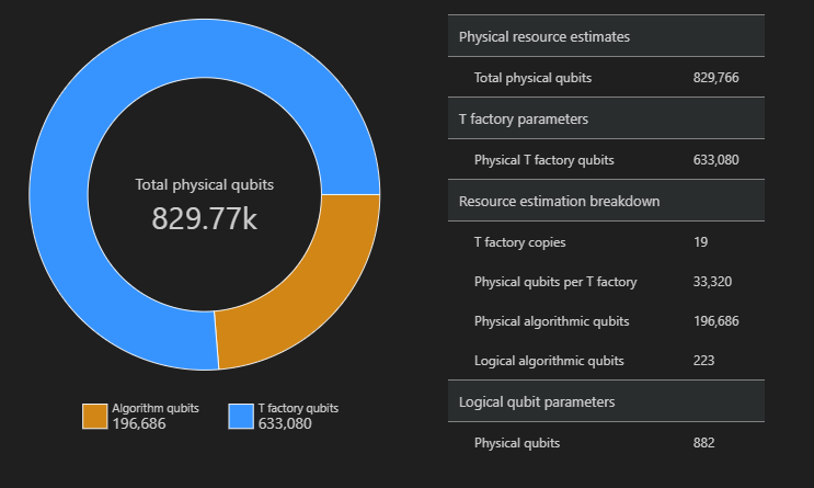
SpaceChart(result)
Bu örnekte, algoritmayı çalıştırmak için gereken fiziksel kubit sayısı 829766 196686 algoritma kubitleri ve 633080'i T fabrika kubitleridir.
Varsayılan değerleri değiştirme ve algoritmayı tahmin
Programınız için bir kaynak tahmini isteği gönderirken bazı isteğe bağlı parametreler belirtebilirsiniz. jobParams İş yürütmeye geçirilebilen tüm target parametrelere erişmek ve hangi varsayılan değerlerin varsayıldığını görmek için alanını kullanın:
result['jobParams']
{'errorBudget': 0.001,
 'qecScheme': {'crossingPrefactor': 0.03,
  'errorCorrectionThreshold': 0.01,
  'logicalCycleTime': '(4 * twoQubitGateTime + 2 * oneQubitMeasurementTime) * codeDistance',
  'name': 'surface_code',
  'physicalQubitsPerLogicalQubit': '2 * codeDistance * codeDistance'},
 'qubitParams': {'instructionSet': 'GateBased',
  'name': 'qubit_gate_ns_e3',
  'oneQubitGateErrorRate': 0.001,
  'oneQubitGateTime': '50 ns',
  'oneQubitMeasurementErrorRate': 0.001,
  'oneQubitMeasurementTime': '100 ns',
  'tGateErrorRate': 0.001,
  'tGateTime': '50 ns',
  'twoQubitGateErrorRate': 0.001,
  'twoQubitGateTime': '50 ns'}}
Kaynak Tahmin Aracı'nın qubit_gate_ns_e3 kubit modelini, surface_code hata düzeltme kodunu ve 0,001 hata bütçesini tahmin için varsayılan değerler olarak aldığını görebilirsiniz.
Özelleştirilebilen parametreler şunlardır target :
errorBudget- algoritma için genel izin verilen hata bütçesiqecScheme- kuantum hata düzeltmesi (QEC) şemasıqubitParams- fiziksel kubit parametrelericonstraints- bileşen düzeyindeki kısıtlamalardistillationUnitSpecifications- T fabrikaları damıtma algoritmaları için belirtimlerestimateType- tek veya sınır
Daha fazla bilgi için bkz. Kaynak Tahmin Aracı için hedef parametreler .
Kubit modelini değiştirme
Majorana tabanlı kubit parametresi qubitParamsolan , "qubit_maj_ns_e6" kullanarak aynı algoritmanın maliyetini tahmin edebilirsiniz.
result_maj = qsharp.estimate("RunProgram()", params={
                "qubitParams": {
                    "name": "qubit_maj_ns_e6"
                }})
EstimateDetails(result_maj)
Kuantum hata düzeltme düzenini değiştirme
Aynı örnek için kaynak tahmin işini Majorana tabanlı kubit parametrelerinde sorgulanmış QEC düzeniyle qecSchemeyeniden çalıştırabilirsiniz.
result_maj = qsharp.estimate("RunProgram()", params={
                "qubitParams": {
                    "name": "qubit_maj_ns_e6"
                },
                "qecScheme": {
                    "name": "floquet_code"
                }})
EstimateDetails(result_maj)
Hata bütçesini değiştirme
Ardından aynı kuantum devresini %10 ile errorBudget yeniden çalıştırın.
result_maj = qsharp.estimate("RunProgram()", params={
                "qubitParams": {
                    "name": "qubit_maj_ns_e6"
                },
                "qecScheme": {
                    "name": "floquet_code"
                },
                "errorBudget": 0.1})
EstimateDetails(result_maj)
Kaynak Tahmin Aracı ile toplu işlem
Azure Quantum Kaynak Tahmin Aracı, birden çok parametre yapılandırması target çalıştırmanıza ve sonuçları karşılaştırmanıza olanak tanır. Bu, farklı kubit modellerinin, QEC düzenlerinin veya hata bütçelerinin maliyetini karşılaştırmak istediğinizde kullanışlıdır.
İşlevin parametresine parametre
paramsqsharp.estimatelistesini target geçirerek toplu tahmin gerçekleştirebilirsiniz. Örneğin, aynı algoritmayı varsayılan parametrelerle ve Majorana tabanlı kubit parametreleriyle bir sorgulanmış QEC şemasıyla çalıştırın.result_batch = qsharp.estimate("RunProgram()", params= [{}, # Default parameters { "qubitParams": { "name": "qubit_maj_ns_e6" }, "qecScheme": { "name": "floquet_code" } }]) result_batch.summary_data_frame(labels=["Gate-based ns, 10⁻³", "Majorana ns, 10⁻⁶"])Modelleme Mantıksal kubitler Mantıksal derinlik T durumları Kod uzaklığı T fabrikaları T fabrika kesri Fiziksel kubitler rQOPS Fiziksel çalışma zamanı Kapı tabanlı ns, 10⁻³ 223 3,64M 4,70M 21 19 76.30 % 829,77k 26,55M 31 sn Majorana ns, 10⁻⁶ 223 3,64M 4,70M 5 19 63.02 % 79.60k 148,67M 5 sn Ayrıca, sınıfını kullanarak
EstimatorParamstahmin parametrelerinin listesini de oluşturabilirsiniz.from qsharp.estimator import EstimatorParams, QubitParams, QECScheme, LogicalCounts labels = ["Gate-based µs, 10⁻³", "Gate-based µs, 10⁻⁴", "Gate-based ns, 10⁻³", "Gate-based ns, 10⁻⁴", "Majorana ns, 10⁻⁴", "Majorana ns, 10⁻⁶"] params = EstimatorParams(num_items=6) params.error_budget = 0.333 params.items[0].qubit_params.name = QubitParams.GATE_US_E3 params.items[1].qubit_params.name = QubitParams.GATE_US_E4 params.items[2].qubit_params.name = QubitParams.GATE_NS_E3 params.items[3].qubit_params.name = QubitParams.GATE_NS_E4 params.items[4].qubit_params.name = QubitParams.MAJ_NS_E4 params.items[4].qec_scheme.name = QECScheme.FLOQUET_CODE params.items[5].qubit_params.name = QubitParams.MAJ_NS_E6 params.items[5].qec_scheme.name = QECScheme.FLOQUET_CODEqsharp.estimate("RunProgram()", params=params).summary_data_frame(labels=labels)Modelleme Mantıksal kubitler Mantıksal derinlik T durumları Kod uzaklığı T fabrikaları T fabrika kesri Fiziksel kubitler rQOPS Fiziksel çalışma zamanı Kapı tabanlı μs, 10⁻³ 223 3,64M 4,70M 17 13 40.54 % 216,77k 21,86k 10 saat Kapı tabanlı μs, 10⁻⁴ 223 3,64M 4,70M 9 14 43.17 % 63,57k 41.30k 5 saat Kapı tabanlı ns, 10⁻³ 223 3,64M 4,70M 17 16 69.08 % 416,89k 32,79M 25 sn Kapı tabanlı ns, 10⁻⁴ 223 3,64M 4,70M 9 14 43.17 % 63,57k 61,94M 13 saniye Majorana ns, 10⁻⁴ 223 3,64M 4,70M 9 19 82.75 % 501.48k 82,59M 10 sn Majorana ns, 10⁻⁶ 223 3,64M 4,70M 5 13 31.47 % 42,96k 148,67M 5 sn
Pareto sınır tahmini çalıştırma
Bir algoritmanın kaynaklarını tahmin ederken, fiziksel kubit sayısı ile algoritmanın çalışma zamanı arasındaki dengeyi göz önünde bulundurmak önemlidir. Algoritmanın çalışma zamanını azaltmak için mümkün olduğunca çok sayıda fiziksel kubit ayırmayı düşünebilirsiniz. Ancak, fiziksel kubitlerin sayısı kuantum donanımında bulunan fiziksel kubit sayısıyla sınırlıdır.
Pareto sınır tahmini, aynı algoritma için her biri kubit sayısı ile çalışma zamanı arasında bir denge olan birden çok tahmin sağlar.
Kaynak Tahmin Aracı'nı Pareto sınır tahmini kullanarak çalıştırmak için parametresini
"estimateType"target olarak"frontier"belirtmeniz gerekir. Örneğin, Pareto sınır tahmini kullanarak bir yüzey koduyla Majorana tabanlı kubit parametreleriyle aynı algoritmayı çalıştırın.result = qsharp.estimate("RunProgram()", params= {"qubitParams": { "name": "qubit_maj_ns_e4" }, "qecScheme": { "name": "surface_code" }, "estimateType": "frontier", # frontier estimation } )işlevini kullanarak
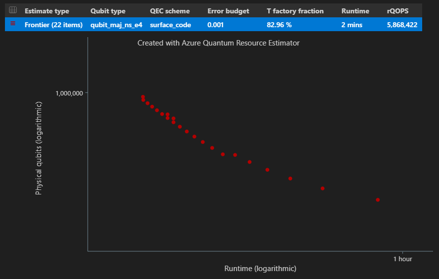
EstimatesOverviewgenel fiziksel kaynak sayılarına sahip bir tablo görüntüleyebilirsiniz. Görüntülemek istediğiniz sütunları seçmek için ilk satırın yanındaki simgeye tıklayın. Çalıştırma adı, tahmin türü, kubit türü, qec şeması, hata bütçesi, mantıksal kubitler, mantıksal derinlik, kod uzaklığı, T durumları, T fabrikaları, T fabrika kesri, çalışma zamanı, rQOPS ve fiziksel kubitler arasından seçim yapabilirsiniz.from qsharp_widgets import EstimatesOverview EstimatesOverview(result)
Sonuçlar tablosunun Tahmin türü sütununda, algoritmanız için farklı {kubit sayısı, çalışma zamanı} birleşimi sayısını görebilirsiniz. Bu durumda Kaynak Tahmin Aracı, binlerce olası kombinasyondan 22 farklı en uygun kombinasyon bulur.
Uzay-zaman diyagramı
EstimatesOverview İşlev ayrıca Kaynak Tahmin Aracı'nın uzay-zaman diyagramını da görüntüler.
Uzay-zaman diyagramı her {kubit sayısı, çalışma zamanı} çifti için fiziksel kubit sayısını ve algoritmanın çalışma zamanını gösterir. Bu noktada kaynak tahmininin ayrıntılarını görmek için her noktanın üzerine gelebilirsiniz.
Pareto sınır tahmini ile toplu işlem
Birden çok parametre yapılandırmasını target sınır tahminiyle tahmin etmek ve karşılaştırmak için parametrelere ekleyin
"estimateType": "frontier",.result = qsharp.estimate( "RunProgram()", [ { "qubitParams": { "name": "qubit_maj_ns_e4" }, "qecScheme": { "name": "surface_code" }, "estimateType": "frontier", # Pareto frontier estimation }, { "qubitParams": { "name": "qubit_maj_ns_e6" }, "qecScheme": { "name": "floquet_code" }, "estimateType": "frontier", # Pareto frontier estimation }, ] ) EstimatesOverview(result, colors=["#1f77b4", "#ff7f0e"], runNames=["e4 Surface Code", "e6 Floquet Code"])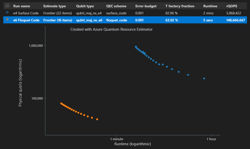
Not
işlevini kullanarak
EstimatesOverviewkubit zamanı diyagramı için renkleri tanımlayabilir ve adları çalıştırabilirsiniz.Pareto sınır tahminini kullanarak birden çok parametre yapılandırması target çalıştırırken, her {kubit sayısı, çalışma zamanı} çifti için olan belirli bir uzay-zaman diyagramı noktası için kaynak tahminlerini görebilirsiniz. Örneğin, aşağıdaki kod ikinci (tahmin dizini=0) çalıştırması ve dördüncü (nokta dizini=3) en kısa çalışma zamanı için tahmin ayrıntıları kullanımını gösterir.
EstimateDetails(result[1], 4)Ayrıca, uzay-zaman diyagramının belirli bir noktasına ait alan diyagramını da görebilirsiniz. Örneğin, aşağıdaki kod ilk birleşim çalıştırması (tahmin dizini=0) ve üçüncü en kısa çalışma zamanı (nokta dizini=2) için alan diyagramını gösterir.
SpaceChart(result[0], 2)
Qiskit için önkoşullar
- Etkin aboneliği olan bir Azure hesabı. Azure hesabınız yoksa ücretsiz kaydolun ve kullandıkça öde aboneliğine kaydolun.
- Azure Quantum çalışma alanı. Daha fazla bilgi için bkz. Azure Quantum çalışma alanını İçerik Oluşturucu.
Çalışma alanınızda Azure Quantum Kaynak Tahmin Aracı'nı target etkinleştirme
Kaynak Tahmin Aracı, Microsoft Quantum Computing sağlayıcısından biridir target . Kaynak Tahmin Aracı'nın yayınlanmasından bu yana bir çalışma alanı oluşturduysanız, Microsoft Quantum Computing sağlayıcısı çalışma alanınıza otomatik olarak eklenir.
Mevcut bir Azure Quantum çalışma alanını kullanıyorsanız:
- çalışma alanınızı Azure portal açın.
- Sol paneldeki İşlemler'in altında Sağlayıcılar'ı seçin.
- + Sağlayıcı ekle'yi seçin.
- Microsoft Quantum Computing için + Ekle'yi seçin.
- Öğren & Geliştir'i ve ekle'yi seçin.
Çalışma alanınızda yeni bir not defteri İçerik Oluşturucu
- Azure portal oturum açın ve Azure Quantum çalışma alanınızı seçin.
- İşlemler'in altında Not Defterleri'ni seçin
- Not defterlerim'e tıklayın ve Yeni Ekle'ye tıklayın
- Çekirdek Türü'ndeIPython'u seçin.
- Dosya için bir ad yazın ve İçerik Oluşturucu dosyasına tıklayın.
Yeni not defteriniz açıldığında, aboneliğinize ve çalışma alanı bilgilerinize göre ilk hücrenin kodunu otomatik olarak oluşturur.
from azure.quantum import Workspace
workspace = Workspace (
    resource_id = "", # Your resource_id
    location = ""  # Your workspace location (for example, "westus")
)
Not
Aksi belirtilmedikçe, derleme sorunlarını önlemek için her hücreyi oluştururken sırayla çalıştırmanız gerekir.
Kodu çalıştırmak için hücrenin solundaki üçgen "oynat" simgesine tıklayın.
Gerekli içeri aktarmaları yükleme
İlk olarak azure-quantum ve qiskit'den ek modüller içeri aktarmanız gerekir.
+ Kod'a tıklayarak yeni bir hücre ekleyin ve aşağıdaki kodu ekleyin ve çalıştırın:
from azure.quantum.qiskit import AzureQuantumProvider
from qiskit import QuantumCircuit, transpile
from qiskit.circuit.library import RGQFTMultiplier
Azure Quantum hizmetine bağlanma
Ardından, Azure Quantum çalışma alanınıza bağlanmak için önceki hücredeki nesneyi kullanarak workspace bir AzureQuantumProvider nesnesi oluşturun. Bir arka uç örneği oluşturur ve Kaynak Tahmin Aracı'nı olarak ayarlarsınız target.
provider = AzureQuantumProvider(workspace)
backend = provider.get_backend('microsoft.estimator')
Kuantum algoritmasını İçerik Oluşturucu
Bu örnekte, Aritmetik uygulamak için Quantum Fourier Dönüşümünü kullanan Ruiz-Perez ve Garcia-Escartin (arXiv:1411.5949) içinde sunulan yapıyı temel alan bir çarpan için kuantum devresi oluşturacaksınız.
Değişkeni değiştirerek bitwidth çarpanın boyutunu ayarlayabilirsiniz. Devre oluşturma, çarpan değeriyle bitwidth çağrılabilen bir işlevde sarmalanır. İşlemin her biri belirtilen boyutuna sahip iki giriş yazmaçları ve belirtilen bitwidthdeğerinin iki katı boyutunda bitwidthbir çıkış yazmaçları olacaktır. İşlev ayrıca doğrudan kuantum devresinden ayıklanan çarpan için bazı mantıksal kaynak sayılarını yazdırır.
def create_algorithm(bitwidth):
    print(f"[INFO] Create a QFT-based multiplier with bitwidth {bitwidth}")

    # Print a warning for large bitwidths that will require some time to generate and
    # transpile the circuit.
    if bitwidth > 18:
        print(f"[WARN] It will take more than one minute generate a quantum circuit with a bitwidth larger than 18")

    circ = RGQFTMultiplier(num_state_qubits=bitwidth, num_result_qubits=2 * bitwidth)

    # One could further reduce the resource estimates by increasing the optimization_level,
    # however, this will also increase the runtime to construct the algorithm.  Note, that
    # it does not affect the runtime for resource estimation.
    print(f"[INFO] Decompose circuit into intrinsic quantum operations")

    circ = transpile(circ, basis_gates=SUPPORTED_INSTRUCTIONS, optimization_level=0)

    # print some statistics
    print(f"[INFO]   qubit count: {circ.num_qubits}")
    print("[INFO]   gate counts")
    for gate, count in circ.count_ops().items():
        print(f"[INFO]   - {gate}: {count}")

    return circ
Not
T durumu olmayan ancak en az bir ölçümü olan algoritmalar için fiziksel kaynak tahmin işleri gönderebilirsiniz.
Kuantum algoritmasını tahmin
işlevini kullanarak algoritmanızın bir örneğini create_algorithm İçerik Oluşturucu. Değişkeni değiştirerek bitwidth çarpanın boyutunu ayarlayabilirsiniz.
bitwidth = 4

circ = create_algorithm(bitwidth)
Varsayılan varsayımları kullanarak bu işlemin fiziksel kaynaklarını tahmin edin. Yöntemini kullanarak bağlantı hattını Kaynak Tahmin Aracı arka ucuna run gönderebilir ve ardından işin tamamlanmasını bekleyip sonuçları döndürmek için komutunu çalıştırabilirsiniz job.result() .
job = backend.run(circ)
result = job.result()
result
Bu, genel fiziksel kaynak sayılarını gösteren bir tablo oluşturur. Daha fazla bilgi içeren grupları daraltarak maliyet ayrıntılarını inceleyebilirsiniz.
İpucu
Çıkış tablosunun daha kompakt bir sürümü için kullanabilirsiniz result.summary.
Örneğin, Mantıksal kubit parametreleri grubunu daraltıyorsanız hata düzeltme kodu uzaklığı değerinin 15 olduğunu daha kolay görebilirsiniz.
| Mantıksal kubit parametresi | Değer |
|---|---|
| QEC şeması | surface_code |
| Kod uzaklığı | 15 |
| Fiziksel kubitler | 450 |
| Mantıksal döngü süresi | 6us |
| Mantıksal kubit hata oranı | 3.00E-10 |
| Ön düzenlemeyi geçme | 0.03 |
| Hata düzeltme eşiği | 0.01 |
| Mantıksal döngü zaman formülü | (4 * twoQubitGateTime + 2 * oneQubitMeasurementTime) * codeDistance |
| Fiziksel kubitler formülü | 2 * codeDistance * codeDistance |
Fiziksel kubit parametreleri grubunda, bu tahmin için varsayılan fiziksel kubit özelliklerini görebilirsiniz. Örneğin, tek kubitli ölçüm ve tek kubitli kapı gerçekleştirme süresinin sırasıyla 100 ns ve 50 ns olduğu varsayılır.
İpucu
Resource Estimator'ın çıkışına result.data() yöntemini kullanarak Python sözlüğü olarak da erişebilirsiniz.
Daha fazla bilgi için Kaynak Tahmin Aracı'nın çıkış verilerinin tam listesine bakın.
Boşluk diyagramları
Algoritma ve T fabrikaları için kullanılan fiziksel kubitlerin dağılımı, algoritmanızın tasarımını etkileyebilecek bir faktördür. Algoritma için tahmini alan gereksinimlerini daha iyi anlamak için bu dağıtımı görselleştirebilirsiniz.
result.diagram.space
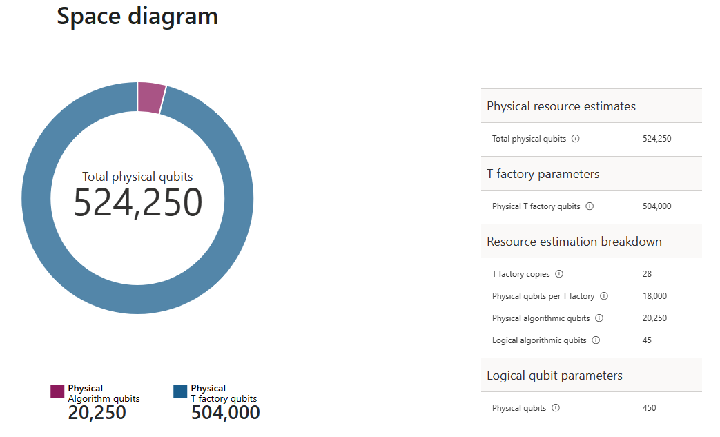
Boşluk diyagramında algoritma kubitlerinin ve T fabrika kubitlerinin oranı gösterilir. 28 numaralı T fabrikası kopyalarının sayısının, T fabrikaları için fiziksel kubit sayısına $\text{T factory} \cdot \text{T factory başına fiziksel kubit}= 28 \cdot 18.000 = 504.000$ olarak katkıda bulunduğunu unutmayın.
Daha fazla bilgi için bkz. T fabrika fiziksel tahmini.
Varsayılan değerleri değiştirme ve algoritmayı tahmin
Programınız için bir kaynak tahmini isteği gönderirken bazı isteğe bağlı parametreler belirtebilirsiniz. jobParams İş yürütmesine geçirilebilen tüm değerlere erişmek ve hangi varsayılan değerlerin varsayıldığını görmek için alanını kullanın:
result.data()["jobParams"]
{'errorBudget': 0.001,
 'qecScheme': {'crossingPrefactor': 0.03,
  'errorCorrectionThreshold': 0.01,
  'logicalCycleTime': '(4 * twoQubitGateTime + 2 * oneQubitMeasurementTime) * codeDistance',
  'name': 'surface_code',
  'physicalQubitsPerLogicalQubit': '2 * codeDistance * codeDistance'},
 'qubitParams': {'instructionSet': 'GateBased',
  'name': 'qubit_gate_ns_e3',
  'oneQubitGateErrorRate': 0.001,
  'oneQubitGateTime': '50 ns',
  'oneQubitMeasurementErrorRate': 0.001,
  'oneQubitMeasurementTime': '100 ns',
  'tGateErrorRate': 0.001,
  'tGateTime': '50 ns',
  'twoQubitGateErrorRate': 0.001,
  'twoQubitGateTime': '50 ns'}}
Özelleştirilebilen parametreler şunlardır target :
errorBudget- izin verilen genel hata bütçesiqecScheme- kuantum hata düzeltmesi (QEC) şemasıqubitParams- fiziksel kubit parametrelericonstraints- bileşen düzeyindeki kısıtlamalardistillationUnitSpecifications- T fabrikaları damıtma algoritmaları için belirtimler
Daha fazla bilgi için bkz. Kaynak Tahmin Aracı için hedef parametreleri .
Kubit modelini değiştirme
Ardından, Majorana tabanlı kubit parametresini kullanarak aynı algoritmanın maliyetini tahmin edin qubit_maj_ns_e6
job = backend.run(circ,
    qubitParams={
        "name": "qubit_maj_ns_e6"
    })
result = job.result()
result
Fiziksel sayıları program aracılığıyla inceleyebilirsiniz. Örneğin, algoritmayı yürütmek için oluşturulan T fabrikası hakkındaki ayrıntıları inceleyebilirsiniz.
result.data()["tfactory"]
{'eccDistancePerRound': [1, 1, 5],
 'logicalErrorRate': 1.6833177305222897e-10,
 'moduleNamePerRound': ['15-to-1 space efficient physical',
  '15-to-1 RM prep physical',
  '15-to-1 RM prep logical'],
 'numInputTstates': 20520,
 'numModulesPerRound': [1368, 20, 1],
 'numRounds': 3,
 'numTstates': 1,
 'physicalQubits': 16416,
 'physicalQubitsPerRound': [12, 31, 1550],
 'runtime': 116900.0,
 'runtimePerRound': [4500.0, 2400.0, 110000.0]}
Not
Çalışma zamanı varsayılan olarak nanosaniye olarak gösterilir.
T fabrikalarının gerekli T durumlarını nasıl ürettiğine ilişkin bazı açıklamalar oluşturmak için bu verileri kullanabilirsiniz.
data = result.data()
tfactory = data["tfactory"]
breakdown = data["physicalCounts"]["breakdown"]
producedTstates = breakdown["numTfactories"] * breakdown["numTfactoryRuns"] * tfactory["numTstates"]

print(f"""A single T factory produces {tfactory["logicalErrorRate"]:.2e} T states with an error rate of (required T state error rate is {breakdown["requiredLogicalTstateErrorRate"]:.2e}).""")
print(f"""{breakdown["numTfactories"]} copie(s) of a T factory are executed {breakdown["numTfactoryRuns"]} time(s) to produce {producedTstates} T states ({breakdown["numTstates"]} are required by the algorithm).""")
print(f"""A single T factory is composed of {tfactory["numRounds"]} rounds of distillation:""")
for round in range(tfactory["numRounds"]):
    print(f"""- {tfactory["numModulesPerRound"][round]} {tfactory["moduleNamePerRound"][round]} unit(s)""")
A single T factory produces 1.68e-10 T states with an error rate of (required T state error rate is 2.77e-08).
23 copies of a T factory are executed 523 time(s) to produce 12029 T states (12017 are required by the algorithm).
A single T factory is composed of 3 rounds of distillation:
- 1368 15-to-1 space efficient physical unit(s)
- 20 15-to-1 RM prep physical unit(s)
- 1 15-to-1 RM prep logical unit(s)
Kuantum hata düzeltme düzenini değiştirme
Şimdi, Aynı örnek için Kaynak tahmini işini Majorana tabanlı kubit parametrelerinde sorgulanmış QEC düzeniyle qecSchemeyeniden çalıştırın.
job = backend.run(circ,
    qubitParams={
        "name": "qubit_maj_ns_e6"
    },
    qecScheme={
        "name": "floquet_code"
    })
result_maj_floquet = job.result()
result_maj_floquet
Hata bütçesini değiştirme
Şimdi aynı kuantum devresini %10 ile errorBudget yeniden çalıştıralım.
job = backend.run(circ,
    qubitParams={
        "name": "qubit_maj_ns_e6"
    },
    qecScheme={
        "name": "floquet_code"
    },
    errorBudget=0.1)
result_maj_floquet_e1 = job.result()
result_maj_floquet_e1
Not
Kaynak Tahmin Aracı ile çalışırken herhangi bir sorunla karşılaşırsanız Sorun Giderme sayfasına göz atın veya ile iletişime geçin AzureQuantumInfo@microsoft.com.
Sonraki adımlar
Geri Bildirim
Çok yakında: 2024 boyunca, içerik için geri bildirim mekanizması olarak GitHub Sorunları’nı kullanımdan kaldıracak ve yeni bir geri bildirim sistemiyle değiştireceğiz. Daha fazla bilgi için bkz. https://aka.ms/ContentUserFeedback.
Gönderin ve geri bildirimi görüntüleyin