End-to-End Predictive Model in AzureML using Linear Regression

Bài viết
11/15/2014

Machine Learning (ML) is one of the most popular field in Computer Science discipline, but is also the most feared by developers. The fear is primarily because it is considered as a scientific field that requires deep mathematical expertise which most of us have forgotten. In today's world, ML has two disciplines: ML, and Applied ML. My goal is to make Machine Learning easier to understand for developers through simple applications. In other words, bridge the gap between a developer and a data scientist. In this blog, I will provide you with a step-by-step guide for building a Linear Regression model in AzureML to predict the price of a car. You will also learn the basics of AzureML along the way, as well as its application it in real-world by creating a Windows Universal Client app.

What is AzureML?

AzureML is meant to democratize Machine Learning and build a new ecosystem and marketplace for monetizing algorithms. You can find more information about AzureML here.

Why AzureML?

Because it is one of the simplest tools to use for Machine Learning. AzureML reduces the barriers to entry for anyone who wants to try out Machine Learning. You don’t have to be a data scientist to build Machine Learning models anymore.

Logical Machine Learning Flow

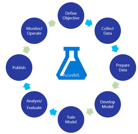
Figure below illustrates a typical machine learning process with end result in mind.

1) Define Objective: Machine Learning is useless without a clear objective for the experiment. Once the objective is clear, then you need to search for the data. In this exercise, our objective is to predict the price of a car based on some attributes provided by an end-user.

2) Collect Data: During this phase, you vehemently collect and ingest the data into a data repository. For this exercise, we will use a sample automobile dataset from the University of California, Irvine’s Machine Learning Repository.

https://archive.ics.uci.edu/ml/datasets/Automobile

Note: This dataset is old and the values no longer represent the values of today’s cars. In a future article, I will show how to feed a real-world automobile feed into the model.

3) Prepare Data: In this phase, you prepare the data for modeling by identifying the features in the dataset. Flatten the data to represent one row per record, remove any outliers, and split the data for training and testing your models. Sometimes, you may have to normalize the data.

4) Develop Model: Designing a model is the fun part, especially using popular ML modeling tool like AzureML, Weka, Lionoso, Orange, MatLab, Octave, R studio, etc. When you develop a model, you feed the data to one or more ML algorithms you have selected for your experiment. In our experiment, we have “true/valid” data and the output will be the predicted price of the car i.e. real-number (or continuous value).

5) Train Model: Typically, supervised learning models need to be trained with data that has already been validated. For example, the car data that we have is “true” data and the output will be a predicted singular value. During training, the ML model operates on the training dataset and builds a pattern that will be used for processing the test and live datasets. You must always keep training and testing datasets separate with minimal overlap.

6) Analyze/Evaluate: Once the model is trained, you can then score the model to generate evaluation metrics and pass it for evaluation. During evaluation, you validate the performance of your trained model and decide whether you want to proceed with it or make adjustments. This is where the experiment gets interesting. If you are not happy with the evaluation, you can readjust the features, change your algorithm for comparison, or even start a brand new experiment.

7) Monitor/Operate: This is where AzureML adds value and empowers not only a data scientist, but also a developer to quickly Publish, Monitor, and even Monetize their algorithms.

Now, lets follow the process described above to build our experiment.

Create Workspace

Navigate your browser to https://www.azure.com and under Feature section, select Analytics –> Machine Learning or go directly here.

Click on Get Started.

There are three steps to start working on AzureML.

You need an Azure account. Microsoft offers free 3 month trials and it is the best way to get started on any Azure service. Once you have an account, login to the Azure Portal.

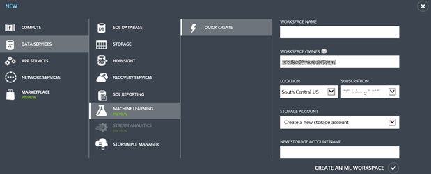
Create a new Machine Learning workspace. New –>Data Services –> Machine Learning

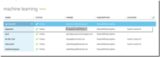
A workspace is used as a collection of experiments that you will be working on. Your workspace should show up in the list of machine learning workspaces. Click on your workspace to go to the ML dashboard.

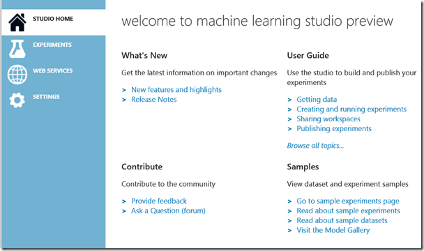
On the dashboard, client on Sign-in to ML Studio. The ML Studio is where you will create your experiments and torture the data.

We have not setup our ML tool for creating experiments. This is just one time setup and now you are free to create as many experiments as you wish. Referring back to our ML flow, we only defined the objective, now we need to collect the data.

Upload Dataset

First download imports-85.data the automobile dataset from https://archive.ics.uci.edu/ml/datasets/Automobile

This data is old, but the purpose is to learn the tool. In a future blog I will show how to get a stream of automobile data and then predict prices based on that.

Click on New-> Dataset –> From Local File

Note: In AzureML, you can also read a dataset from a URL directly into your experiment. By uploading the dataset you are saving it for future use.

Create a new Experiment

Click on New –> Experiment –> Blank Experiment

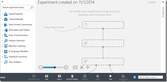
This will create a new experiment canvas with a tool box on the left for you to drag and drop components

Connect Data

Your Automobile dataset should appear in the Saved Datasets section of the toolbox. Drag and drop the automobile data onto the canvas.

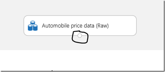
Note that the data component has a connection point to connect to other components. If you have used any Workflow or ETL tools before, this should sound familiar to you.

Prepare Data

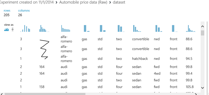
I usually follow the best practice to test my experiment at every stage and on every change I make. So, right-click on the connection point and client Visualize to see the list of raw automobile data.

But, there is a problem. Some of the data is missing. This might create adverse effects in predicting the car value. And we also don’t need the normalized-losses column (feature) for prediction purposes. That column is used for insurance information. So, to get rid of that column, drag Project Columns component from Data Transformation –> Manipulation.

Project Columns component lets you filter the columns from one stage to another. In our case, we will not project the normalized-losses column at all.

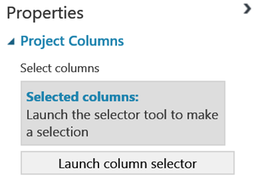
Next, click the Launch column selector from the Properties (right-side ) pane

In the Select Columns window, select “All columns” to select all columns and then select “Exclude” –> “column names”, and add “normalized-losses” as shown in the figure below.

To validate, save the project, and Visualize the Project Column’s output connection point.

If you observe carefully, there are some missing values in some columns and these values may create unnecessary noise in our prediction, therefore, let’s remove all the rows containing missing values.

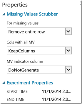
To remove missing values, drag the missing values scrubber and connect Project Columns to Missing Values Scrubber. Select “Remove entire row” from the “For missing values” dropdown list.

Next, Save, Run and Visualize to validate whether your dataset consists of all the values. Note the number of rows and columns displayed to compare them with the original dataset.

Now, we have scrubbed the dataset, but considering our objective of predicting the car price, there are still many columns that may not be a contributing factor to the price of a car. A simple question I would is: “What affects the price of a car?”. Now, remember that this is an experiment and your answer will be different than mine. My hypothesis is that the following columns from the dataset affect the price of a car.

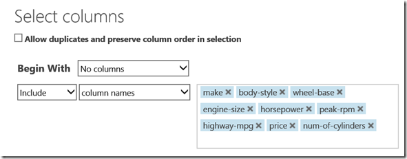
make, body-style, wheel-base, engine-size, horsepower, peak-rpm, highway-mpg, num-of-cylinders

Add another Project Columns component, Launch Column selector and select the listed columns to project.

Run and Visualize the data. You should see only the selected columns displayed.

Split Data

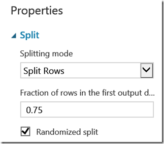
The data is now prepared to be fed to the model. But, in ML, you must first train the model and then test the hypothesis with test data that is different from the training data. AzureML provides you with a Split function to split the data into two paths. Add the Split component and connect it to the Project Columns as shown in the Figure below.

It is a common practice to split the data 75% (training) and 25% (testing).

Train a Linear Regression Model

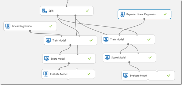
Next, drag the Linear Regression, Train Model, and Score Model components. The Score Model component generates predictions on the test data by using the trained model. Connect the Linear Regression and Split components to the Train Model. Select the price column as the outcome column. The outcome column consists the predicted value.

Connect the Train Model to the Score Model. Next, connect the second output of the Split component to the Score Model. The output of the Score Model is sent to the Evaluate Model component for generating Evaluation metrics. The finished model looks like the figure below.

Run the model and Visualize the Evaluate node. The Evaluation results will consist of a table with the following columns:

Coefficient of Determination (R2): Determines how well your regression line fits the statistical data. The value of R2 is between 0 and 1 with 1 being a perfect fit. In our case, R2 is approximately 82%. Whether this value is good or bad depends on the error tolerance for your output. In automobile prediction, I am happy with 82% success. If you want to improve the results further, you can modify the Project Columns and also the settings for the Liner Regression. You may also try another algorithm like Bayesian Linear Regression. You can either create a new experiment or add Bayesian Linear Regression component to the current experiment and feed it exactly the same data as before.

When you run the experiment, it runs both the models and evaluation is done separately. In our experiment, R2 came out to be 89%.

Now assuming that we are happy with the model’s results, lets publish the model as a web service to that you can access it from anywhere.

Save the Trained Models

Right-Click on the Linear Regression and Bayesian Trained Model components and select “Save as Trained Model”. We are saving the model to be reused by other programs.

The saved models should show up in the Trained Models list

Now you can use these trained models with live data within your applications.

Prepare Model for Web Service

To prepare your model for two web services, SAVE AS the original experiment two times as:

1) Auto Prediction Linear Regression

2) Auto Prediction Bayesian Linear Regression

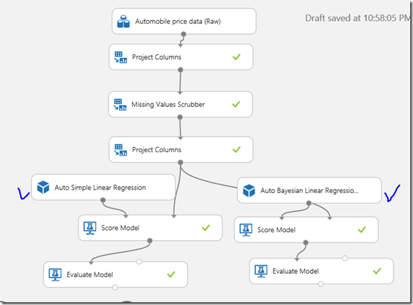
Next replace the Linear Regression, Bayesian Linear Regression and their associated Train Model components with our saved models as illustrated below. Run an visualize both the Evaluation Model results.

Evaluation for Linear Regression

Evaluation Results for Bayesian Linear Regression

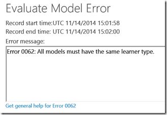
Note: Typically, you would point both the regressions to the same evaluate model, but the constraint for the Evaluate model to compare both regressions is that they must have the same learner type. Bayesian is a more probabilistic method than linear fit, thus the error.

I did this on purpose for you to understand the capabilities and constraints of AzureML. But, you could instead use Poisson Regression model and evaluate it with Linear Regression.

You can now Visualize the Evaluate Model to compare the Coefficient of Determination.

You an also see the liner fits and prediction performance by visualizing the Score Model.

For the web service, let’s publish the Bayesian Linear Regression because the R2 value looks consistently better than the Linear Regression.

One thing to not forget here is that you can always go back, test the results and publish only when you are satisfied.

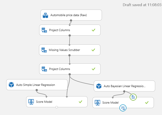
Rick-Click the Score Model input endpoint for Bayesian Linear Regression and select “Set as Publish Input”. Next, Right-Click the output endpoint of the Score Model and select “Set as Publish Output”. These two settings specify the data input and output for the web service calls. The final model should look like the figure below.

Finally, after running the model once again, the Publish Web Service button will be enabled. Click on it to proceed with web service publishing to a staging environment.

Testing the Webservice

On the Dashboard, you should see the API Key, and Test link for testing the web service. You can enter the car details for price prediction.

Input Data: audi sedan 99.8 four 109 102 5500 30 13950

Predicted Price: 12732

Publish Webservice to Production

By default, the web service is created in a staging environment. If you are happy with the prediction, let’s move ahead with publishing the web service to production.

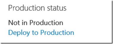
Click “Mark as Ready for Production” link in the Production status section.

Next, in the settings section, select “YES” and click Save.

Next, go back to the Dashboard and click “Deploy to Production” to go to the AzureML webservices page

Click on Add to create the web service in the region of your choice.

The web service gets deployed in seconds (if not minutes). Click on the web service and you will be navigated to the web service management dashboard where you will be able to see the REQUEST/RESPONSE as well as BATCH EXECUTION endpoints for the web service.

Click on the REQUEST/RESPONSE link to go to the endpoint documentation page. On this page you will find the client signatures for C#, R, and Python, and also the input JSON request.

Sample JSON Request

 {
  "Id": "score00001",
  "Instance": {
    "FeatureVector": {
      "make": "0",
      "body-style": "0",
      "wheel-base": "0",
      "num-of-cylinders": "0",
      "engine-size": "0",
      "horsepower": "0",
      "peak-rpm": "0",
      "highway-mpg": "0",
      "price": "0"
    },
    "GlobalParameters": {}
  }
}

C# Client Code

// This code requires the Nuget package Microsoft.AspNet.WebApi.Client to be installed. // Instructions for doing this in Visual Studio: // Tools -> Nuget Package Manager -> Package Manager Console // Install-Package Microsoft.AspNet.WebApi.Client using System; using System.Collections.Generic; using System.IO; using System.Net.Http; using System.Net.Http.Formatting; using System.Net.Http.Headers; using System.Text; using System.Threading.Tasks; namespace CallRequestResponseService { public class ScoreData { public Dictionary<string, string> FeatureVector { get; set; } public Dictionary<string, string> GlobalParameters { get; set; } } public class ScoreRequest { public string Id { get; set; } public ScoreData Instance { get; set; } } class Program { static void Main(string[] args) { InvokeRequestResponseService().Wait(); } static async Task InvokeRequestResponseService() { using (var client = new HttpClient()) { ScoreData scoreData = new ScoreData() { FeatureVector = new Dictionary<string, string>() { { "make", "0" }, { "body-style", "0" }, { "wheel-base", "0" }, { "num-of-cylinders", "0" }, { "engine-size", "0" }, { "horsepower", "0" }, { "peak-rpm", "0" }, { "highway-mpg", "0" }, { "price", "0" }, }, GlobalParameters = new Dictionary<string, string>() { } }; ScoreRequest scoreRequest = new ScoreRequest() { Id = "score00001", Instance = scoreData }; const string apiKey = "abc123"; // Replace this with the API key for the web service client.DefaultRequestHeaders.Authorization = new AuthenticationHeaderValue("Bearer", apiKey); client.BaseAddress = new Uri("https://ussouthcentral.services.azureml.net/xxxxb62/score"); HttpResponseMessage response = await client.PostAsJsonAsync("", scoreRequest); if (response.IsSuccessStatusCode) { string result = await response.Content.ReadAsStringAsync(); Console.WriteLine("Result: {0}", result); } else { Console.WriteLine("Failed with status code: {0}", response.StatusCode); } } } } }

With the C# Client and REST interface, you can call the web service from any PC, Mobile, and Web clients.

Let’s build a Mobile App

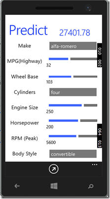
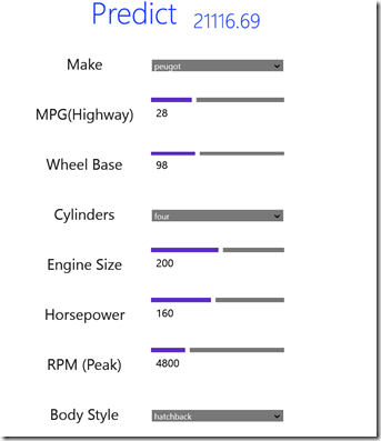
With the web service running in Azure, there is no reason not to build a mobile app user interface. I just quickly put together a Windows Universal App to predict car prices. You can find the source code for the app here.

Conclusion

AzureML is a new and highly productive tool for Machine Learning. It may be the only tool that lets you publish a machine learning web service directly from your design environment. Machine Learning is a vast topic and Linear Regression models discussed in this article only scratches the surface of the topic. In this article, I went over a stale dataset to showcase AzureML as a predictive analytics tool. You can apply the same procedures and components for Classification and Clustering models. Finally, my goal was in writing about Applied Machine Learning. I am not a Data Scientist, but now with all the productive tools, I feel that I can put to work some of the great algorithms that scientists have already invented.

Some more Datasets you can play around with

References

https://www.mathworks.com/help/stats/multiple-linear-regression-1.html?refresh=true
https://horicky.blogspot.com/2012/05/predictive-analytics-generalized-linear.html
https://horicky.blogspot.com/2012/05/predictive-analytics-overview-and-data.html
https://101.datascience.community/2013/03/07/9-problems-with-real-world-regression/
https://blogs.msdn.com/b/continuous_learning/