Microsoft Fabric 中的笔记本可视化效果

2025-05-26

Microsoft Fabric 是一种集成的分析服务，可加速跨数据仓库和大数据系统快速获得见解。笔记本中的数据可视化是一项关键功能，可用于深入了解数据，帮助用户轻松识别模式、趋势和离群值。

使用 Fabric 中的 Apache Spark 时，可以使用内置选项来可视化数据，包括 Fabric 笔记本图表功能和对常用开源库的访问。

Fabric 笔记本还允许你将表格结果转换为自定义图表，而无需编写任何代码，从而提供更直观和无缝的数据浏览体验。

内置可视化命令 - display() 函数

借助 Fabric 内置可视化函数，可以将 Apache Spark 数据帧、Pandas 数据帧和 SQL 查询结果转换为丰富的交互式数据可视化效果。

使用显示函数，可以将 PySpark 和 Scala Spark 数据帧或弹性分布式数据集（RDD）呈现为动态表或图表。

可以指定要呈现的数据帧的行计数。默认值为 1000。笔记本显示输出小组件最多支持查看和分析 10000 行数据帧。

可以使用全局工具栏上的筛选器函数对数据应用自定义规则。筛选条件应用于指定列，结果将同时反映在表视图和图表视图中。

默认情况下，SQL 语句的输出使用与 display() 相同的控件。

丰富的数据帧表视图

表视图上的自由选择支持

默认情况下，在 Fabric 笔记本中使用 display（） 命令时，将呈现表视图。丰富的数据帧预览提供了直观的免费选择功能，旨在通过启用灵活的交互式选择选项来增强数据分析体验。此功能允许用户轻松导航和浏览数据帧。

列选择
- 单列：单击列标题以选择整个列。
- 多个列：选择单个列后，按住“Shift”键，然后单击另一列标题以选择多个列。
行选择
- 单行：单击行标题以选择整行。
- 多行：选择单行后，按住“Shift”键，然后单击另一行标题以选择多行。
单元格内容预览：预览各个单元格的内容，以便快速详细地查看数据，而无需编写其他代码。
列摘要：获取每个列（包括数据分布和关键统计信息）的摘要，以便快速了解数据的特征。
可用区域选择：选择表格的任何连续段，大致了解所选单元格总数和选定区域中的数值。
复制所选内容：在所有选择情况下，可以使用“Ctrl + C”快捷方式快速复制所选内容。所选数据以 CSV 格式复制，便于在其他应用程序中处理。

通过“检查窗格”的数据分析支持

丰富数据帧预览的动态 GIF。

可通过单击“检查”按钮来分析数据帧。它提供汇总的数据分布，并会显示每一列的统计信息。
“检查”侧窗格的每个卡片映射到数据帧的一列，可通过单击卡片或选择表中的一列来查看更多详细信息。
可通过单击表中的单元格查看单元格详细信息。当数据帧包含长字符串类型的内容时，此功能非常有用。

增强型丰富的数据框架图表视图

display（） 命令中改进的图表视图提供了更直观和动态的方式来可视化数据。

关键增强功能：

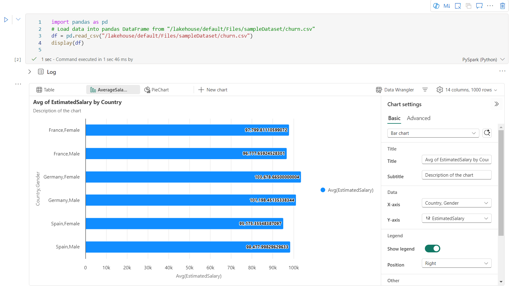
多图表支持：通过选择“新建图表”，在单个显示（）输出小组件中最多添加五个图表，从而实现跨不同列的轻松比较。
智能图表建议：根据数据帧获取建议的图表列表。选择编辑建议的可视化效果，或从头开始创建自定义图表。

灵活定制：个性化您的可视化效果，设置可根据所选图表类型进行调整。

类别	基本设置	描述
	图表类型	display 函数支持多种图表类型，包括条形图、散点图、折线图、数据透视表等。
标题	标题	图表的标题。
标题	副标题	显示更多说明的图表副标题。
数据	X 轴	指定图表的键。
数据	Y 轴	指定图表的值。
图例	显示图例	启用/禁用图例。
图例	位置	自定义图例的位置。
其他	序列组	使用此配置确定聚合的组。
其他	聚合	使用此方法可聚合可视化效果中的数据。
其他	堆叠	配置结果的显示样式。
其他	缺失值和空值	配置显示缺失或 NULL 图表值的方式。

注意

此外，还可以指定显示的行数，默认设置为 1,000。笔记本显示输出小组件支持查看和分析最多 10,000 行的数据帧。选择“聚合所有结果”，然后选择“应用”以应用根据整个数据帧生成的图表。图表设置更改时会触发 Spark 作业。完成计算并呈现图表可能需要几分钟时间。

类别	高级设置	描述
颜色	主题	定义图表的主题颜色集。
X 轴	标签	指定 X 轴的标签。
X 轴	缩放	指定 X 轴的 scale 函数。
X 轴	范围	指定 X 轴的值范围。
Y 轴	标签	指定 Y 轴的标签。
Y 轴	缩放	指定 Y 轴的 scale 函数。
Y 轴	范围	指定 Y 轴的值范围。
显示	显示标签	显示/隐藏图表上的结果标签。

配置更改会立即生效，所有配置都会自动保存在笔记本内容中。

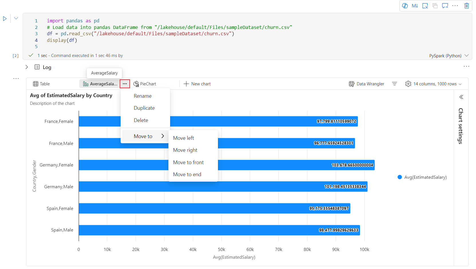
可以在图表选项卡菜单中轻松 重命名、重复、删除或移动图表。还可以拖放选项卡以对其重新排序。打开笔记本时，第一个选项卡将显示为默认值。
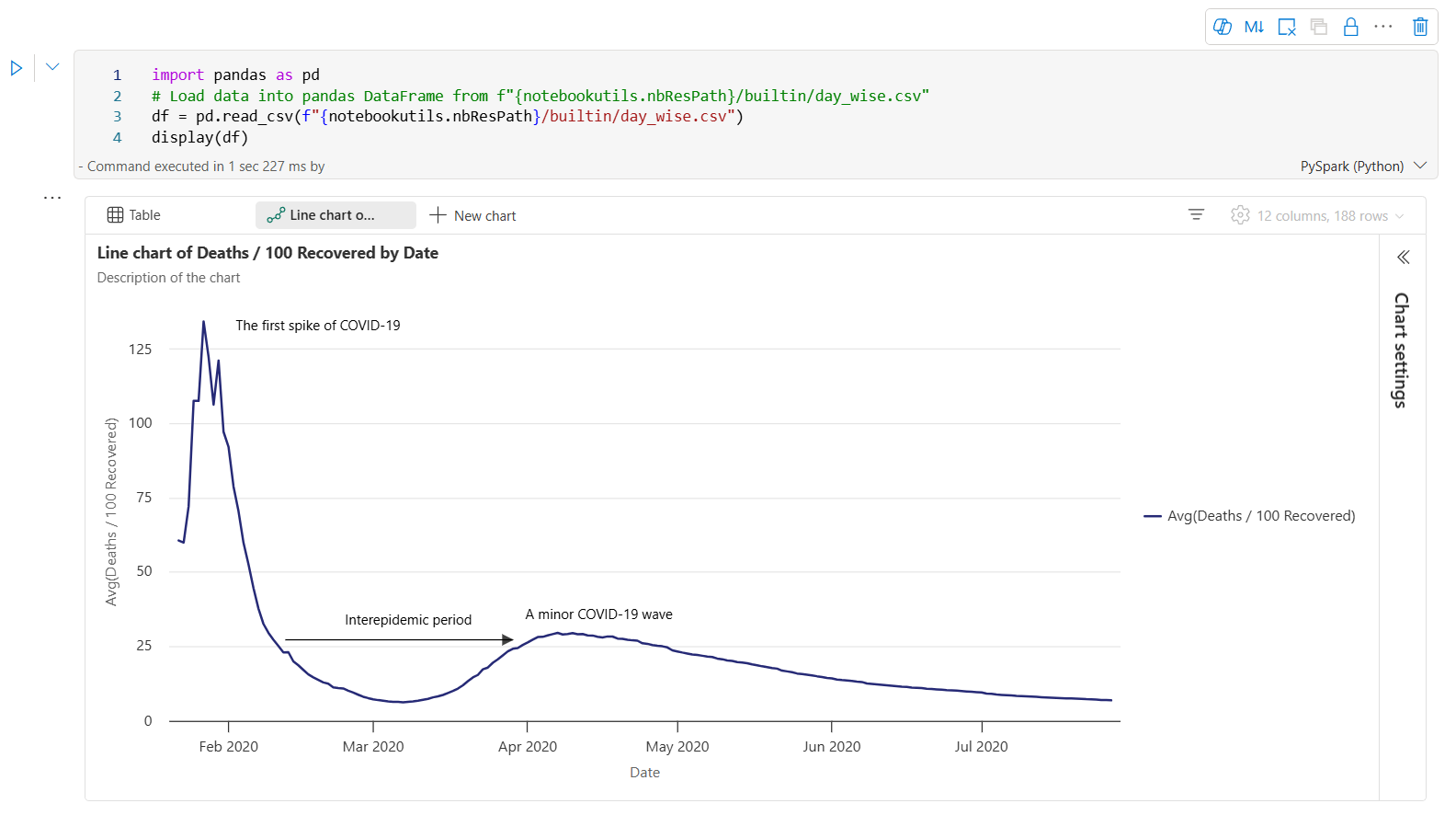
当用户将鼠标悬停在图表上时，新的图表体验中提供了交互式工具栏。支持放大、缩小、选定区域放大、重置、平移、批注编辑等操作。

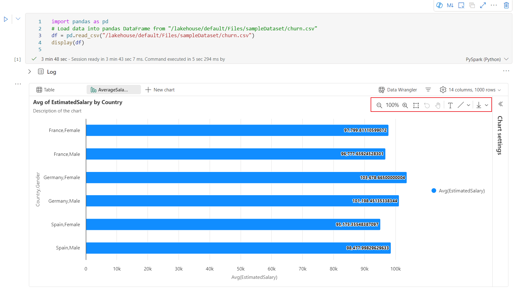
下面是图表批注的示例。

display() 摘要视图

使用 display(df, summary = true) 检查给定 Apache Spark 数据帧的统计信息摘要。摘要包括每列的列名、列类型、唯一值和缺失值。你还可以选择特定列来查看其最小值、最大值、平均值和标准差。

摘要视图的动画 GIF。

displayHTML() 选项

Fabric 笔记本支持使用 displayHTML 函数的 HTML 图形。

下图是使用 D3.js 创建可视化效果的示例。

要创建此可视化效果，可运行以下代码。

displayHTML("""<!DOCTYPE html>
<meta charset="utf-8">

<!-- Load d3.js -->
<script src="https://d3js.org/d3.v4.js"></script>

<!-- Create a div where the graph will take place -->
<div id="my_dataviz"></div>
<script>

// set the dimensions and margins of the graph
var margin = {top: 10, right: 30, bottom: 30, left: 40},
  width = 400 - margin.left - margin.right,
  height = 400 - margin.top - margin.bottom;

// append the svg object to the body of the page
var svg = d3.select("#my_dataviz")
.append("svg")
  .attr("width", width + margin.left + margin.right)
  .attr("height", height + margin.top + margin.bottom)
.append("g")
  .attr("transform",
        "translate(" + margin.left + "," + margin.top + ")");

// Create Data
var data = [12,19,11,13,12,22,13,4,15,16,18,19,20,12,11,9]

// Compute summary statistics used for the box:
var data_sorted = data.sort(d3.ascending)
var q1 = d3.quantile(data_sorted, .25)
var median = d3.quantile(data_sorted, .5)
var q3 = d3.quantile(data_sorted, .75)
var interQuantileRange = q3 - q1
var min = q1 - 1.5 * interQuantileRange
var max = q1 + 1.5 * interQuantileRange

// Show the Y scale
var y = d3.scaleLinear()
  .domain([0,24])
  .range([height, 0]);
svg.call(d3.axisLeft(y))

// a few features for the box
var center = 200
var width = 100

// Show the main vertical line
svg
.append("line")
  .attr("x1", center)
  .attr("x2", center)
  .attr("y1", y(min) )
  .attr("y2", y(max) )
  .attr("stroke", "black")

// Show the box
svg
.append("rect")
  .attr("x", center - width/2)
  .attr("y", y(q3) )
  .attr("height", (y(q1)-y(q3)) )
  .attr("width", width )
  .attr("stroke", "black")
  .style("fill", "#69b3a2")

// show median, min and max horizontal lines
svg
.selectAll("toto")
.data([min, median, max])
.enter()
.append("line")
  .attr("x1", center-width/2)
  .attr("x2", center+width/2)
  .attr("y1", function(d){ return(y(d))} )
  .attr("y2", function(d){ return(y(d))} )
  .attr("stroke", "black")
</script>

"""
)

在笔记本中嵌入 Power BI 报表

重要

此功能目前为预览版。

Powerbiclient Python 包现在在 Fabric 笔记本中原生受支持。无需在 Fabric 笔记本 Spark 运行时 3.4 上执行任何额外的设置（例如身份验证过程）。只需导入 powerbiclient，然后即可继续探索。若要详细了解如何使用 powerbiclient 包，请参阅 powerbiclient 文档。

Powerbiclient 支持以下关键功能。

呈现现有的 Power BI 报表

只需几行代码即可轻松地在笔记本中嵌入 Power BI 报表并与之交互。

下图是呈现现有 Power BI 报表的示例。

运行以下代码来呈现现有的 Power BI 报表。

from powerbiclient import Report

report_id="Your report id"
report = Report(group_id=None, report_id=report_id)

report

从 Spark 数据帧创建报表视觉对象

可以在笔记本中使用 Spark 数据帧快速生成见解可视化效果。还可以选择“保存”嵌入报表，以在目标工作区中创建报表项。

下图是来自 Spark 数据帧的 QuickVisualize() 的示例。

运行以下代码以从 Spark 数据帧呈现报表。

# Create a spark dataframe from a Lakehouse parquet table
sdf = spark.sql("SELECT * FROM testlakehouse.table LIMIT 1000")

# Create a Power BI report object from spark data frame
from powerbiclient import QuickVisualize, get_dataset_config
PBI_visualize = QuickVisualize(get_dataset_config(sdf))

# Render new report
PBI_visualize

从 pandas 数据帧创建报表视觉对象

还可以基于笔记本中的 pandas 数据帧创建报表。

下图是来自 pandas 数据帧的 QuickVisualize() 的示例。

运行以下代码以从 Spark 数据帧呈现报表。

import pandas as pd

# Create a pandas dataframe from a URL
df = pd.read_csv("https://raw.githubusercontent.com/plotly/datasets/master/fips-unemp-16.csv")

# Create a pandas dataframe from a Lakehouse csv file
from powerbiclient import QuickVisualize, get_dataset_config

# Create a Power BI report object from your data
PBI_visualize = QuickVisualize(get_dataset_config(df))

# Render new report
PBI_visualize

常用库

在数据可视化效果方面，Python 提供了多个图形库，这些库包含许多不同的功能。默认情况下，Fabric 中的每个 Apache Spark 池都包含一组精选和常用的开放源代码库。

Matplotlib

可以使用每个库的内置呈现功能（如 Matplotlib），来呈现标准绘图库。

下图是使用 Matplotlib 创建条形图的示例。

运行下面的示例代码以绘制此条形图。

# Bar chart

import matplotlib.pyplot as plt

x1 = [1, 3, 4, 5, 6, 7, 9]
y1 = [4, 7, 2, 4, 7, 8, 3]

x2 = [2, 4, 6, 8, 10]
y2 = [5, 6, 2, 6, 2]

plt.bar(x1, y1, label="Blue Bar", color='b')
plt.bar(x2, y2, label="Green Bar", color='g')
plt.plot()

plt.xlabel("bar number")
plt.ylabel("bar height")
plt.title("Bar Chart Example")
plt.legend()
plt.show()

散景

可以使用 displayHTML(df) 来呈现 HTML 或交互库，如 bokeh。

下图是使用 bokeh 在地图上绘制字形的示例。

要绘制此图像，可运行下面的示例代码。

from bokeh.plotting import figure, output_file
from bokeh.tile_providers import get_provider, Vendors
from bokeh.embed import file_html
from bokeh.resources import CDN
from bokeh.models import ColumnDataSource

tile_provider = get_provider(Vendors.CARTODBPOSITRON)

# range bounds supplied in web mercator coordinates
p = figure(x_range=(-9000000,-8000000), y_range=(4000000,5000000),
           x_axis_type="mercator", y_axis_type="mercator")
p.add_tile(tile_provider)

# plot datapoints on the map
source = ColumnDataSource(
    data=dict(x=[ -8800000, -8500000 , -8800000],
              y=[4200000, 4500000, 4900000])
)

p.circle(x="x", y="y", size=15, fill_color="blue", fill_alpha=0.8, source=source)

# create an html document that embeds the Bokeh plot
html = file_html(p, CDN, "my plot1")

# display this html
displayHTML(html)

Plotly (数据可视化工具)

你可以使用 displayHTML() 来呈现 HTML 或交互式库，如 Plotly 。