教程:创建、评估文本分类模型并对其评分
本教程介绍了 Microsoft Fabric 中文本分类模型的 Synapse 数据科学工作流的端到端示例。 此方案使用 Spark 上的 word2vec 和逻辑回归,仅根据书名从大英图书馆图书数据集中确定该书的类型。
本教程涵盖以下步骤:
- 安装自定义库
- 加载数据
- 通过探索性数据分析来理解和处理数据
- 使用 word2vec 和逻辑回归训练机器学习模型,并使用 MLflow 和 Fabric 自动记录功能跟踪实验
- 加载机器学习模型进行评分和预测
先决条件
获取 Microsoft Fabric 订阅。 或者注册免费的 Microsoft Fabric 试用版。
登录 Microsoft Fabric。
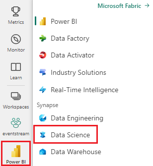
使用主页左侧的体验切换器切换到 Synapse 数据科学体验。
- 如果没有 Microsoft Fabric 湖屋,请按照在 Microsoft Fabric 中创建湖屋中的步骤创建一个。
在笔记本中进行操作
可以选择下面其中一个选项,以在笔记本中进行操作:
- 在 Synapse 数据科学体验中打开并运行内置笔记本
- 将笔记本从 GitHub 上传到 Synapse 数据科学体验
打开内置笔记本
本教程附带示例标题流派分类笔记本。
若要在 Synapse 数据科学体验中打开教程的内置示例笔记本,请执行以下操作:
转到 Synapse 数据科学主页。
选择“使用示例”。
选择相应的示例:
- 来自默认的“端到端工作流 (Python)”选项卡(如果示例适用于 Python 教程)。
- 来自“端到端工作流 (R)“选项卡(如果示例适用于 R 教程)。
- 从“快速教程”选项卡选择(如果示例适用于快速教程)。
从 GitHub 导入笔记本
AIsample - Title Genre Classification.ipynb 是本教程随附的笔记本。
若要打开本教程随附的笔记本,请按照让系统为数据科学做好准备教程中的说明操作,将该笔记本导入到工作区。
或者,如果要从此页面复制并粘贴代码,则可以创建新的笔记本。
在开始运行代码之前,请务必将湖屋连接到笔记本。
步骤 1:安装自定义库
对于机器学习模型开发或临时数据分析,可能需要为 Apache Spark 会话快速安装自定义库。 有两个选项可用于安装库。
- 使用笔记本的内联安装功能(
%pip或%conda),仅在当前笔记本中安装库。 - 也可以创建 Fabric 环境,安装来自公共来源的安装库或将自定义库上传到该环境,然后工作区管理员可以将环境附加为工作区的默认值。 然后,环境中的所有库都将可用于工作区中的任何笔记本和 Spark 作业定义。 有关环境的详细信息,请参阅在 Microsoft Fabric 中创建、配置和使用环境。
对于分类模型,使用 wordcloud 库来表示文本中单词的频率,即用单词的大小代表其频率。 本教程将使用 %pip install 在笔记本中安装 wordcloud。
注意
PySpark 内核将在 %pip install 之后重启。 在运行任何其他单元之前安装所需的库。
# Install wordcloud for text visualization by using pip
%pip install wordcloud
步骤 2:加载数据
该数据集包含有关大英图书馆与 Microsoft 合作进行数字化的大英图书馆书籍的元数据。 元数据是分类信息,用于指示书籍是小说还是非小说。 此数据集旨在训练一个根据书名即可确定书籍类型的分类模型。
| BL 记录 ID | 资源的类型 | 名称 | 与名称关联的日期 | 名称类型 | 角色 | 所有名称 | 标题 | 变体标题 | 系列标题 | 系列内的编号 | 出版国家/地区 | 出版地点 | 发布者 | 发布日期 | 版本 | 物理描述 | 杜威分类法 | BL 货架标记 | 主题 | 流派 | 语言 | 说明 | 物理资源的 BL 记录 ID | classification_id | user_id | created_at | subject_ids | annotator_date_pub | annotator_normalised_date_pub | annotator_edition_statement | annotator_genre | annotator_FAST_genre_terms | annotator_FAST_subject_terms | annotator_comments | annotator_main_language | annotator_other_languages_summaries | annotator_summaries_language | annotator_translation | annotator_original_language | annotator_publisher | annotator_place_pub | annotator_country | annotator_title | 数字化书籍的链接 | 已批注 |
|---|---|---|---|---|---|---|---|---|---|---|---|---|---|---|---|---|---|---|---|---|---|---|---|---|---|---|---|---|---|---|---|---|---|---|---|---|---|---|---|---|---|---|---|---|---|
| 014602826 | 专著 | Yearsley, Ann | 1753-1806 | 个人 | More, Hannah, 1745-1833 [person]; Yearsley, Ann, 1753-1806 [person] | 几个场合的诗歌 [附有 Hannah More 的前言信]。 | 英格兰 | London | 1786 | 第四版手稿备注 | Digital Store 11644.d.32 | 英语 | 003996603 | 错误 | |||||||||||||||||||||||||||||||
| 014602830 | 专著 | A, T. | 个人 | Oldham, John, 1653-1683 [person]; A, T. [person] | A Satyr against Vertue. (一首诗:应该是由 Town-Hector 说的 [John Oldham 著。序言署名:T. A.]) | 英格兰 | London | 1679 | 15 页 (4°) | Digital Store 11602.ee.10. (2.) | 英语 | 000001143 | False |
定义以下参数,以便可以将此笔记本应用于不同的数据集:
IS_CUSTOM_DATA = False  # If True, the user must manually upload the dataset
DATA_FOLDER = "Files/title-genre-classification"
DATA_FILE = "blbooksgenre.csv"

# Data schema
TEXT_COL = "Title"
LABEL_COL = "annotator_genre"
LABELS = ["Fiction", "Non-fiction"]

EXPERIMENT_NAME = "sample-aisample-textclassification"  # MLflow experiment name
下载数据集并上传到湖屋
以下代码将下载数据集的公开可用版本,然后将其存储在 Fabric 湖屋中。
重要
在运行笔记本之前,请将湖屋添加到笔记本。 否则可能会导致出错。
if not IS_CUSTOM_DATA:
    # Download demo data files into the lakehouse, if they don't exist
    import os, requests

    remote_url = "https://synapseaisolutionsa.blob.core.windows.net/public/Title_Genre_Classification"
    fname = "blbooksgenre.csv"
    download_path = f"/lakehouse/default/{DATA_FOLDER}/raw"

    if not os.path.exists("/lakehouse/default"):
        # Add a lakehouse, if no default lakehouse was added to the notebook
        # A new notebook won't link to any lakehouse by default
        raise FileNotFoundError(
            "Default lakehouse not found, please add a lakehouse and restart the session."
        )
    os.makedirs(download_path, exist_ok=True)
    if not os.path.exists(f"{download_path}/{fname}"):
        r = requests.get(f"{remote_url}/{fname}", timeout=30)
        with open(f"{download_path}/{fname}", "wb") as f:
            f.write(r.content)
    print("Downloaded demo data files into lakehouse.")
导入所需的库
在进行任何处理之前,需要先导入所需的库,包括 Spark 和 SynapseML 的库:
import numpy as np
from itertools import chain

from wordcloud import WordCloud
import matplotlib.pyplot as plt
import seaborn as sns

import pyspark.sql.functions as F

from pyspark.ml import Pipeline
from pyspark.ml.feature import *
from pyspark.ml.tuning import CrossValidator, ParamGridBuilder
from pyspark.ml.classification import LogisticRegression
from pyspark.ml.evaluation import (
    BinaryClassificationEvaluator,
    MulticlassClassificationEvaluator,
)

from synapse.ml.stages import ClassBalancer
from synapse.ml.train import ComputeModelStatistics

import mlflow
定义超参数
定义一些用于模型训练的超参数。
重要
仅当你了解每个参数时才修改这些超参数。
# Hyperparameters
word2vec_size = 128  # The length of the vector for each word
min_word_count = 3  # The minimum number of times that a word must appear to be considered
max_iter = 10  # The maximum number of training iterations
k_folds = 3  # The number of folds for cross-validation
开始记录运行此笔记本所需的时间:
# Record the notebook running time
import time

ts = time.time()
设置 MLflow 试验跟踪
自动记录将扩展 MLflow 日志记录功能。 自动记录会在你训练机器学习模型时自动捕获该模型的输入参数值和输出指标。 然后,你可以将此信息记录到工作区。 在工作区中,你可以使用 MLflow API 或工作区中的相应试验来访问和可视化信息。 要了解自动记录的更多信息,请参阅 Microsoft Fabric 中的自动记录。
# Set up Mlflow for experiment tracking

mlflow.set_experiment(EXPERIMENT_NAME)
mlflow.autolog(disable=True)  # Disable Mlflow autologging
若要在笔记本会话中禁用 Microsoft Fabric 自动日志记录,请调用 mlflow.autolog() 并设置 disable=True:
从湖屋中读取原始日期数据
raw_df = spark.read.csv(f"{DATA_FOLDER}/raw/{DATA_FILE}", header=True, inferSchema=True)
步骤 3:执行探索性数据分析
使用 display 命令探索数据集,以查看数据集的概要统计信息并显示图表视图:
display(raw_df.limit(20))
准备数据
删除重复项以清理数据:
df = (
    raw_df.select([TEXT_COL, LABEL_COL])
    .where(F.col(LABEL_COL).isin(LABELS))
    .dropDuplicates([TEXT_COL])
    .cache()
)

display(df.limit(20))
应用类别平衡来解决任何偏差:
# Create a ClassBalancer instance, and set the input column to LABEL_COL
cb = ClassBalancer().setInputCol(LABEL_COL)

# Fit the ClassBalancer instance to the input DataFrame, and transform the DataFrame
df = cb.fit(df).transform(df)

# Display the first 20 rows of the transformed DataFrame
display(df.limit(20))
将段落和句子拆分为较小的单位,以对数据集进行词汇切分。 这样就能更轻松地分配含义。 然后,删除非索引字以提高性能。 非索引字删除涉及删除语料库所有文档中常见的单词。 非索引字删除是自然语言处理 (NLP) 应用程序中最常用的预处理步骤之一。
# Text transformer
tokenizer = Tokenizer(inputCol=TEXT_COL, outputCol="tokens")
stopwords_remover = StopWordsRemover(inputCol="tokens", outputCol="filtered_tokens")

# Build the pipeline
pipeline = Pipeline(stages=[tokenizer, stopwords_remover])

token_df = pipeline.fit(df).transform(df)

display(token_df.limit(20))
显示每个类的词云库。 词云库是文本数据中频繁出现的关键字的视觉突出呈现。 词云库之所以有效,是因为关键字的呈现形成了云状的彩色图片,可以更好地一目了然地捕获主要文本数据。 详细了解词云。
# WordCloud
for label in LABELS:
    tokens = (
        token_df.where(F.col(LABEL_COL) == label)
        .select(F.explode("filtered_tokens").alias("token"))
        .where(F.col("token").rlike(r"^\w+$"))
    )

    top50_tokens = (
        tokens.groupBy("token").count().orderBy(F.desc("count")).limit(50).collect()
    )

    # Generate a wordcloud image
    wordcloud = WordCloud(
        scale=10,
        background_color="white",
        random_state=42,  # Make sure the output is always the same for the same input
    ).generate_from_frequencies(dict(top50_tokens))

    # Display the generated image by using matplotlib
    plt.figure(figsize=(10, 10))
    plt.title(label, fontsize=20)
    plt.axis("off")
    plt.imshow(wordcloud, interpolation="bilinear")
最后,使用 word2vec 对文本进行矢量化。 word2vec 技术可以为文本中每个单词创建矢量表示形式。 在相似上下文中使用的单词或具有语义关系的单词可以通过它们在矢量空间中的接近度来有效捕获。 这种接近度表明相似的单词具有相似的单词矢量。
# Label transformer
label_indexer = StringIndexer(inputCol=LABEL_COL, outputCol="labelIdx")
vectorizer = Word2Vec(
    vectorSize=word2vec_size,
    minCount=min_word_count,
    inputCol="filtered_tokens",
    outputCol="features",
)

# Build the pipeline
pipeline = Pipeline(stages=[label_indexer, vectorizer])
vec_df = (
    pipeline.fit(token_df)
    .transform(token_df)
    .select([TEXT_COL, LABEL_COL, "features", "labelIdx", "weight"])
)

display(vec_df.limit(20))
步骤 4:训练和评估模型
数据就位后,定义模型。 在此部分,需要训练一个逻辑回归模型来对矢量化的文本进行分类。
准备训练和测试数据集
# Split the dataset into training and testing
(train_df, test_df) = vec_df.randomSplit((0.8, 0.2), seed=42)
跟踪机器学习试验
机器学习试验是组织和控制所有相关机器学习运行的主要单元。 一次运行对应于模型代码的单次执行。
机器学习试验跟踪管理所有实验及其组件,例如参数、指标、模型和其他项目。 跟踪可以组织特定机器学习试验的所有必需组件。 它还可以通过保存的试验轻松重现过去的结果。 详细了解 Microsoft Fabric 中的机器学习试验。
# Build the logistic regression classifier
lr = (
    LogisticRegression()
    .setMaxIter(max_iter)
    .setFeaturesCol("features")
    .setLabelCol("labelIdx")
    .setWeightCol("weight")
)
优化超参数
构建参数网格以搜索超参数。 然后构建交叉计算器估算器,以生成 CrossValidator 模型:
# Build a grid search to select the best values for the training parameters
param_grid = (
    ParamGridBuilder()
    .addGrid(lr.regParam, [0.03, 0.1])
    .addGrid(lr.elasticNetParam, [0.0, 0.1])
    .build()
)

if len(LABELS) > 2:
    evaluator_cls = MulticlassClassificationEvaluator
    evaluator_metrics = ["f1", "accuracy"]
else:
    evaluator_cls = BinaryClassificationEvaluator
    evaluator_metrics = ["areaUnderROC", "areaUnderPR"]
evaluator = evaluator_cls(labelCol="labelIdx", weightCol="weight")

# Build a cross-evaluator estimator
crossval = CrossValidator(
    estimator=lr,
    estimatorParamMaps=param_grid,
    evaluator=evaluator,
    numFolds=k_folds,
    collectSubModels=True,
)
评估模型
我们可以利用数据集对模型进行评测,从而对其进行比较。 针对验证数据集和测试数据集运行时,经过良好训练的模型应该在相关指标上表现出高性能。
def evaluate(model, df):
    log_metric = {}
    prediction = model.transform(df)
    for metric in evaluator_metrics:
        value = evaluator.evaluate(prediction, {evaluator.metricName: metric})
        log_metric[metric] = value
        print(f"{metric}: {value:.4f}")
    return prediction, log_metric
使用 MLflow 跟踪试验
启动训练和产品评测流程。 使用 MLflow 跟踪所有试验并记录参数、指标和模型。 所有这些信息都记录在工作区中的试验名称下。
with mlflow.start_run(run_name="lr"):
    models = crossval.fit(train_df)
    best_metrics = {k: 0 for k in evaluator_metrics}
    best_index = 0
    for idx, model in enumerate(models.subModels[0]):
        with mlflow.start_run(nested=True, run_name=f"lr_{idx}") as run:
            print("\nEvaluating on test data:")
            print(f"subModel No. {idx + 1}")
            prediction, log_metric = evaluate(model, test_df)

            if log_metric[evaluator_metrics[0]] > best_metrics[evaluator_metrics[0]]:
                best_metrics = log_metric
                best_index = idx

            print("log model")
            mlflow.spark.log_model(
                model,
                f"{EXPERIMENT_NAME}-lrmodel",
                registered_model_name=f"{EXPERIMENT_NAME}-lrmodel",
                dfs_tmpdir="Files/spark",
            )

            print("log metrics")
            mlflow.log_metrics(log_metric)

            print("log parameters")
            mlflow.log_params(
                {
                    "word2vec_size": word2vec_size,
                    "min_word_count": min_word_count,
                    "max_iter": max_iter,
                    "k_folds": k_folds,
                    "DATA_FILE": DATA_FILE,
                }
            )

    # Log the best model and its relevant metrics and parameters to the parent run
    mlflow.spark.log_model(
        models.subModels[0][best_index],
        f"{EXPERIMENT_NAME}-lrmodel",
        registered_model_name=f"{EXPERIMENT_NAME}-lrmodel",
        dfs_tmpdir="Files/spark",
    )
    mlflow.log_metrics(best_metrics)
    mlflow.log_params(
        {
            "word2vec_size": word2vec_size,
            "min_word_count": min_word_count,
            "max_iter": max_iter,
            "k_folds": k_folds,
            "DATA_FILE": DATA_FILE,
        }
    )
查看试验:
- 在左侧导航窗格中选择你的工作区
- 查找并选择试验名称,在本例中为 sample_aisample-textclassification

步骤 5:对预测结果评分并将其保存
Microsoft Fabric 允许用户通过 PREDICT 可缩放函数来操作机器学习模型。 此函数支持任何计算引擎中的批处理评分(或批处理推理)。 你可以直接从笔记本或特定模型的项页创建批量预测。 若要了解有关 PREDICT 以及如何在 Fabric 中使用它的更多信息,请参阅在 Microsoft Fabric 中使用 PREDICT 进行机器学习模型评分。
从上述产品评测结果来看,模型 1 具有最大的精准率-召回率曲线下面积 (AUPRC) 和接收者操作特性曲线下面积 (AUC-ROC) 指标。 因此你应该使用模型 1 进行预测。
AUC-ROC 度量值广泛用于度量二元分类器的性能。 然而,有时,根据 AUPRC 度量值来评测分类器更为合适。 AUC-ROC 图表直观显示了真正率 (TPR) 和假正率 (FPR) 之间的权衡。 AUPRC 是一条在单个可视化效果中结合了精准率(正预测值,简称 PPV)和召回率(真正率,简称 TPR)的曲线。
# Load the best model
model_uri = f"models:/{EXPERIMENT_NAME}-lrmodel/1"
loaded_model = mlflow.spark.load_model(model_uri, dfs_tmpdir="Files/spark")

# Verify the loaded model
batch_predictions = loaded_model.transform(test_df)
batch_predictions.show(5)
# Code to save userRecs in the lakehouse
batch_predictions.write.format("delta").mode("overwrite").save(
    f"{DATA_FOLDER}/predictions/batch_predictions"
)
# Determine the entire runtime
print(f"Full run cost {int(time.time() - ts)} seconds.")
相关内容
反馈
即将发布:在整个 2024 年,我们将逐步淘汰作为内容反馈机制的“GitHub 问题”,并将其取代为新的反馈系统。 有关详细信息,请参阅:https://aka.ms/ContentUserFeedback。
提交和查看相关反馈