注意
为了获得更大的功能, PyTorch 还可用于 Windows 上的 DirectML。
在本教程的前一阶段中,我们获取了将用于使用 PyTorch 训练图像分类器的数据集。 现在,是时候利用这些数据了。
要使用 PyTorch 训练图像分类器,需要完成以下步骤:
- 加载数据。 如果你已经完成了本教程的上一步,那么你已经处理过这个了。
- 定义卷积神经网络。
- 定义损失函数。
- 使用训练数据训练模型。
- 使用测试数据测试网络。
定义卷积神经网络。
若要使用 PyTorch 构建神经网络,你将使用 torch.nn 包。 该包包含模块、可扩展类和构建神经网络所需的全部组件。
在本部分中,你将构建一个基本的卷积神经网络 (CNN) 来对 CIFAR10 数据集中的图像进行分类。
CNN 是一类神经网络,定义为多层神经网络,旨在检测数据中的复杂特征。 它们最常用于计算机视觉应用程序。
我们的网络将由以下 14 层构成:
Conv -> BatchNorm -> ReLU -> Conv -> BatchNorm -> ReLU -> MaxPool -> Conv -> BatchNorm -> ReLU -> Conv -> BatchNorm -> ReLU -> Linear。
卷积层
卷积层是 CNN 的主要层,可帮助我们检测图像中的特征。 每个层都有多个通道来检测图像中的特定特征,还有多个内核来定义检测到的特征的大小。 因此,具有 64 个通道和 3 x 3 内核大小的卷积层将检测 64 个不同的特征,每个大小为 3 x 3。 定义卷积层时,需要提供输入通道数、输出通道数和内核大小。 该层中的输出通道数为下一层的输入通道数。
例如:输入通道数为 3、输出通道数为 10、内核大小为 6 的卷积层将得到 RGB 图像(3 通道)作为输入,并对核大小为 6x6 的图像应用 10 个特征检测器。 较小的内核大小将缩短计算时间和权重共享。
其他层
我们的网络还涉及以下其他层:
-
ReLU层是一个激活函数,用于将所有传入特征定义为 0 或更大。 应用此层时,任何小于 0 的数字都会更改为零,而其他数字则保持不变。 -
BatchNorm2d层对输入应用规范化以获得零均值和单位方差并提高网络精度。 -
MaxPool层将帮助我们确保图像中对象的位置不会影响神经网络检测其特定特征的能力。 -
Linear层是网络中的最后一层,它计算每个类的分数。 在 CIFAR10 数据集中,有 10 类标签。 得分最高的标签将是模型预测的那一个。 在线性层中,必须指定输入特征的数量和输出特征的数量,它们应与类的数量相对应。
神经网络如何工作?
CNN 是一种前馈网络。 在训练过程中,网络将处理所有层的输入,计算损失以了解图像的预测标签与正确标签相差多远,并将梯度传播回网络以更新层的权重。 通过迭代庞大的输入数据集,网络将“学习”设置其权重以获得最佳结果。
前向函数计算损失函数的值,后向函数计算可学习参数的梯度。 使用 PyTorch 创建神经网络时,只需定义前向函数。 后向函数会自动定义。
- 将以下代码复制到 Visual Studio 中的
PyTorchTraining.py文件以定义 CCN。
import torch
import torch.nn as nn
import torchvision
import torch.nn.functional as F

# Define a convolution neural network
class Network(nn.Module):
    def __init__(self):
        super(Network, self).__init__()

        self.conv1 = nn.Conv2d(in_channels=3, out_channels=12, kernel_size=5, stride=1, padding=1)
        self.bn1 = nn.BatchNorm2d(12)
        self.conv2 = nn.Conv2d(in_channels=12, out_channels=12, kernel_size=5, stride=1, padding=1)
        self.bn2 = nn.BatchNorm2d(12)
        self.pool = nn.MaxPool2d(2,2)
        self.conv4 = nn.Conv2d(in_channels=12, out_channels=24, kernel_size=5, stride=1, padding=1)
        self.bn4 = nn.BatchNorm2d(24)
        self.conv5 = nn.Conv2d(in_channels=24, out_channels=24, kernel_size=5, stride=1, padding=1)
        self.bn5 = nn.BatchNorm2d(24)
        self.fc1 = nn.Linear(24*10*10, 10)

    def forward(self, input):
        output = F.relu(self.bn1(self.conv1(input)))
        output = F.relu(self.bn2(self.conv2(output)))
        output = self.pool(output)
        output = F.relu(self.bn4(self.conv4(output)))
        output = F.relu(self.bn5(self.conv5(output)))
        output = output.view(-1, 24*10*10)
        output = self.fc1(output)

        return output

# Instantiate a neural network model
model = Network()
注意
想要详细了解如何使用 PyTorch 创建神经网络? 请查看 PyTorch 文档
定义损失函数
损失函数计算一个值,该值可估计输出与目标之间的差距。 主要目标是通过神经网络中的反向传播改变权重向量值来减少损失函数的值。
丢失值不同于模型准确性。 通过损失函数可了解模型在每次训练集优化迭代后的表现。 模型的准确性基于测试数据进行计算,并显示正确预测的百分比。
在 PyTorch 中,神经网络包包含各种损失函数,这些函数构成了深层神经网络的构建基块。 在本教程中,你将先使用分类交叉熵损失定义损失函数和 Adam 优化器,然后再使用分类损失函数。 学习速率 (lr) 设置你根据损失梯度调整网络权重的程度控制。 请将其设置为 0.001。 速率越低,训练速度就越慢。
- 将以下代码复制到 Visual Studio 中的
PyTorchTraining.py文件中,以定义损失函数和优化器。
from torch.optim import Adam

# Define the loss function with Classification Cross-Entropy loss and an optimizer with Adam optimizer
loss_fn = nn.CrossEntropyLoss()
optimizer = Adam(model.parameters(), lr=0.001, weight_decay=0.0001)
使用训练数据训练模型。
要训练模型,必须循环访问数据迭代器,将输入馈送到网络并进行优化。 PyTorch 没有用于 GPU 的专用库,但你可以手动定义执行设备。 如果计算机上存在 Nvidia GPU,则该设备为 Nvidia GPU,如果没有,则为 CPU。
- 将以下代码添加到
PyTorchTraining.py文件
from torch.autograd import Variable

# Function to save the model
def saveModel():
    path = "./myFirstModel.pth"
    torch.save(model.state_dict(), path)

# Function to test the model with the test dataset and print the accuracy for the test images
def testAccuracy():

    model.eval()
    accuracy = 0.0
    total = 0.0
    device = torch.device("cuda:0" if torch.cuda.is_available() else "cpu")

    with torch.no_grad():
        for data in test_loader:
            images, labels = data
            # run the model on the test set to predict labels
            outputs = model(images.to(device))
            # the label with the highest energy will be our prediction
            _, predicted = torch.max(outputs.data, 1)
            total += labels.size(0)
            accuracy += (predicted == labels.to(device)).sum().item()

    # compute the accuracy over all test images
    accuracy = (100 * accuracy / total)
    return(accuracy)


# Training function. We simply have to loop over our data iterator and feed the inputs to the network and optimize.
def train(num_epochs):

    best_accuracy = 0.0

    # Define your execution device
    device = torch.device("cuda:0" if torch.cuda.is_available() else "cpu")
    print("The model will be running on", device, "device")
    # Convert model parameters and buffers to CPU or Cuda
    model.to(device)

    for epoch in range(num_epochs):  # loop over the dataset multiple times
        running_loss = 0.0
        running_acc = 0.0

        for i, (images, labels) in enumerate(train_loader, 0):

            # get the inputs
            images = Variable(images.to(device))
            labels = Variable(labels.to(device))

            # zero the parameter gradients
            optimizer.zero_grad()
            # predict classes using images from the training set
            outputs = model(images)
            # compute the loss based on model output and real labels
            loss = loss_fn(outputs, labels)
            # backpropagate the loss
            loss.backward()
            # adjust parameters based on the calculated gradients
            optimizer.step()

            # Let's print statistics for every 1,000 images
            running_loss += loss.item()     # extract the loss value
            if i % 1000 == 999:
                # print every 1000 (twice per epoch)
                print('[%d, %5d] loss: %.3f' %
                      (epoch + 1, i + 1, running_loss / 1000))
                # zero the loss
                running_loss = 0.0

        # Compute and print the average accuracy fo this epoch when tested over all 10000 test images
        accuracy = testAccuracy()
        print('For epoch', epoch+1,'the test accuracy over the whole test set is %d %%' % (accuracy))

        # we want to save the model if the accuracy is the best
        if accuracy > best_accuracy:
            saveModel()
            best_accuracy = accuracy
使用测试数据测试模型。
现在,可以使用测试集中的一批图像来测试模型。
- 将以下代码添加到
PyTorchTraining.py文件。
import matplotlib.pyplot as plt
import numpy as np

# Function to show the images
def imageshow(img):
    img = img / 2 + 0.5     # unnormalize
    npimg = img.numpy()
    plt.imshow(np.transpose(npimg, (1, 2, 0)))
    plt.show()


# Function to test the model with a batch of images and show the labels predictions
def testBatch():
    # get batch of images from the test DataLoader
    images, labels = next(iter(test_loader))

    # show all images as one image grid
    imageshow(torchvision.utils.make_grid(images))

    # Show the real labels on the screen
    print('Real labels: ', ' '.join('%5s' % classes[labels[j]]
                               for j in range(batch_size)))

    # Let's see what if the model identifiers the  labels of those example
    outputs = model(images)

    # We got the probability for every 10 labels. The highest (max) probability should be correct label
    _, predicted = torch.max(outputs, 1)

    # Let's show the predicted labels on the screen to compare with the real ones
    print('Predicted: ', ' '.join('%5s' % classes[predicted[j]]
                              for j in range(batch_size)))
最后,让我们添加主代码。 这将启动模型训练、保存模型并在屏幕上显示结果。 我们将在训练集上仅运行两次迭代 [train(2)],因此训练过程不会花费太长时间。
- 将以下代码添加到
PyTorchTraining.py文件。
if __name__ == "__main__":

    # Let's build our model
    train(5)
    print('Finished Training')

    # Test which classes performed well
    testAccuracy()

    # Let's load the model we just created and test the accuracy per label
    model = Network()
    path = "myFirstModel.pth"
    model.load_state_dict(torch.load(path))

    # Test with batch of images
    testBatch()
让我们运行测试! 确保顶部工具栏中的下拉菜单设置为“调试”。 将解决方案平台更改为 x64(如果设备是 64 位的)或 x86(如果设备是 32 位的)以在你的本地计算机上运行该项目。
选择等于 2 ([train(2)]) 的时期数(完整通过训练数据集的次数)将导致对包含 10,000 个图像的整个测试数据集进行两次迭代。 在第 8 代 Intel CPU 上完成训练大约需要 20 分钟,该模型对 10 个标签的分类成功率应达到 65% 左右。
- 若要打开项目,请单击工具栏上的“开始调试”按钮,或者按 F5。
控制台窗口将弹出,并显示训练过程。
正如你所定义的那样,将每隔 1,000 批图像打印一次损失值,训练集的每次迭代打印五次。 你希望每个循环的损失值逐渐减少。
还可以在每次迭代后查看模型的准确性。 模型准确性与损失值不同。 通过损失函数可了解模型在每次训练集优化迭代后的表现。 模型的准确性基于测试数据进行计算,并显示正确预测的百分比。 在本例中,它将指示模型在每次训练迭代后能够从 10,000 个图像测试集中正确分类的图像数量。
训练完成后,应会看到类似于下面的输出。 数字不会完全相同 - 训练取决于许多因素,并且不会总是返回相同的结果 - 但它们应该看起来相似。
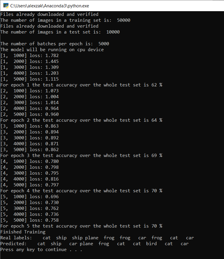
仅运行 5 个时期后,模型成功率为 70%。 对于短期训练的基本模型来说,这是一个很好的结果!
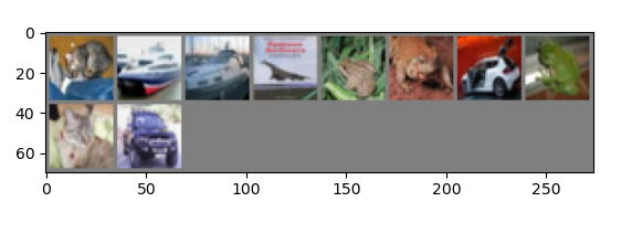
用一批图像进行测试,模型从该批次的 10 个图像中得出了 7 个正确的图像。 结果很不错,与模型成功率一致。
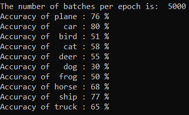
您可以检查我们的模型最擅长预测哪些类别。 只需添加并运行以下代码:
- 可选 - 将以下 函数添加到
testClassess文件中,在主函数PyTorchTraining.py中添加此函数testClassess()的调用__name__ == "__main__"。
# Function to test what classes performed well
def testClassess():
    class_correct = list(0. for i in range(number_of_labels))
    class_total = list(0. for i in range(number_of_labels))
    with torch.no_grad():
        for data in test_loader:
            images, labels = data
            outputs = model(images)
            _, predicted = torch.max(outputs, 1)
            c = (predicted == labels).squeeze()
            for i in range(batch_size):
                label = labels[i]
                class_correct[label] += c[i].item()
                class_total[label] += 1

    for i in range(number_of_labels):
        print('Accuracy of %5s : %2d %%' % (
            classes[i], 100 * class_correct[i] / class_total[i]))
输出如下所示:
后续步骤
现在我们有了一个分类模型,下一步是将模型转换为 ONNX 格式