執行資源估算器的不同方式
在本文中,您將瞭解如何使用 Azure Quantum Resource Estimator。 資源估算器可在 VS Code 和在線 Azure 入口網站 取得。
下表顯示執行資源估算器的不同方式。
| 使用者案例 | 平台 | 教學課程 |
|---|---|---|
| 估計 Q# 計劃的資源 | Visual Studio Code | 在頁面頂端的 VS Code 中選取 Q# |
| 估計 Q# 計劃的資源 (進階) | Visual Studio Code中的 Jupyter Notebook | 選取頁面頂端 Jupyter Notebook 中的 Q# |
| 估計 Qiskit 計劃的資源 | Azure Quantum 入口網站 | 選取頁面頂端 Azure 入口網站 中的 Qiskit |
| 估計 QIR 計劃的資源 | Azure Quantum 入口網站 | 提交 QIR |
| 使用FCIDUMP檔案做為自變數參數, (進階) | Visual Studio Code | 提交量子化學問題 |
注意
2024 年 6 月 30 日之後,將不再支援 Microsoft Quantum Development Kit (傳統 QDK) 。 如果您是現有的 QDK 開發人員,建議您轉換至新的 Azure Quantum Development Kit (Modern QDK) ,以繼續開發量子解決方案。 如需詳細資訊,請參閱 將您的 Q# 程式代碼移轉至新式 QDK。
VS Code 的必要條件
- 最新版的 Visual Studio Code 或開啟網路上的 VS Code。
- 最新版的 Azure Quantum Development Kit 擴充功能。 如需安裝詳細數據,請參閱 在 VS Code 上安裝新式 QDK。
提示
您不需要有 Azure 帳戶才能執行本機資源估算器。
Create 新的 Q# 檔案
- 開啟 Visual Studio Code,然後選取 [檔案>新文本檔] 以建立新的檔案。
- 將檔案儲存為
ShorRE.qs。 此檔案將包含您程式的 Q# 程式代碼。
Create 量子演算法
將下列程式代碼 ShorRE.qs 複製到檔案:
namespace Shors {
    open Microsoft.Quantum.Arrays;
    open Microsoft.Quantum.Canon;
    open Microsoft.Quantum.Convert;
    open Microsoft.Quantum.Diagnostics;
    open Microsoft.Quantum.Intrinsic;
    open Microsoft.Quantum.Math;
    open Microsoft.Quantum.Measurement;
    open Microsoft.Quantum.Unstable.Arithmetic;
    open Microsoft.Quantum.ResourceEstimation;

    @EntryPoint()
    operation RunProgram() : Unit {
        let bitsize = 31;

        // When chooseing parameters for `EstimateFrequency`, make sure that
        // generator and modules are not co-prime
        let _ = EstimateFrequency(11, 2^bitsize - 1, bitsize);
    }

    // In this sample we concentrate on costing the `EstimateFrequency`
    // operation, which is the core quantum operation in Shors algorithm, and
    // we omit the classical pre- and post-processing.

    /// # Summary
    /// Estimates the frequency of a generator
    /// in the residue ring Z mod `modulus`.
    ///
    /// # Input
    /// ## generator
    /// The unsigned integer multiplicative order (period)
    /// of which is being estimated. Must be co-prime to `modulus`.
    /// ## modulus
    /// The modulus which defines the residue ring Z mod `modulus`
    /// in which the multiplicative order of `generator` is being estimated.
    /// ## bitsize
    /// Number of bits needed to represent the modulus.
    ///
    /// # Output
    /// The numerator k of dyadic fraction k/2^bitsPrecision
    /// approximating s/r.
    operation EstimateFrequency(
        generator : Int,
        modulus : Int,
        bitsize : Int
    )
    : Int {
        mutable frequencyEstimate = 0;
        let bitsPrecision =  2 * bitsize + 1;

        // Allocate qubits for the superposition of eigenstates of
        // the oracle that is used in period finding.
        use eigenstateRegister = Qubit[bitsize];

        // Initialize eigenstateRegister to 1, which is a superposition of
        // the eigenstates we are estimating the phases of.
        // We first interpret the register as encoding an unsigned integer
        // in little endian encoding.
        ApplyXorInPlace(1, eigenstateRegister);
        let oracle = ApplyOrderFindingOracle(generator, modulus, _, _);

        // Use phase estimation with a semiclassical Fourier transform to
        // estimate the frequency.
        use c = Qubit();
        for idx in bitsPrecision - 1..-1..0 {
            within {
                H(c);
            } apply {
                // `BeginEstimateCaching` and `EndEstimateCaching` are the operations
                // exposed by Azure Quantum Resource Estimator. These will instruct
                // resource counting such that the if-block will be executed
                // only once, its resources will be cached, and appended in
                // every other iteration.
                if BeginEstimateCaching("ControlledOracle", SingleVariant()) {
                    Controlled oracle([c], (1 <<< idx, eigenstateRegister));
                    EndEstimateCaching();
                }
                R1Frac(frequencyEstimate, bitsPrecision - 1 - idx, c);
            }
            if MResetZ(c) == One {
                set frequencyEstimate += 1 <<< (bitsPrecision - 1 - idx);
            }
        }

        // Return all the qubits used for oracles eigenstate back to 0 state
        // using Microsoft.Quantum.Intrinsic.ResetAll.
        ResetAll(eigenstateRegister);

        return frequencyEstimate;
    }

    /// # Summary
    /// Interprets `target` as encoding unsigned little-endian integer k
    /// and performs transformation |k⟩ ↦ |gᵖ⋅k mod N ⟩ where
    /// p is `power`, g is `generator` and N is `modulus`.
    ///
    /// # Input
    /// ## generator
    /// The unsigned integer multiplicative order ( period )
    /// of which is being estimated. Must be co-prime to `modulus`.
    /// ## modulus
    /// The modulus which defines the residue ring Z mod `modulus`
    /// in which the multiplicative order of `generator` is being estimated.
    /// ## power
    /// Power of `generator` by which `target` is multiplied.
    /// ## target
    /// Register interpreted as little endian encoded which is multiplied by
    /// given power of the generator. The multiplication is performed modulo
    /// `modulus`.
    internal operation ApplyOrderFindingOracle(
        generator : Int, modulus : Int, power : Int, target : Qubit[]
    )
    : Unit
    is Adj + Ctl {
        // The oracle we use for order finding implements |x⟩ ↦ |x⋅a mod N⟩. We
        // also use `ExpModI` to compute a by which x must be multiplied. Also
        // note that we interpret target as unsigned integer in little-endian
        // encoding.
        ModularMultiplyByConstant(modulus,
                                    ExpModI(generator, power, modulus),
                                    target);
    }

    /// # Summary
    /// Performs modular in-place multiplication by a classical constant.
    ///
    /// # Description
    /// Given the classical constants `c` and `modulus`, and an input
    /// quantum register  |𝑦⟩, this operation
    /// computes `(c*x) % modulus` into |𝑦⟩.
    ///
    /// # Input
    /// ## modulus
    /// Modulus to use for modular multiplication
    /// ## c
    /// Constant by which to multiply |𝑦⟩
    /// ## y
    /// Quantum register of target
    internal operation ModularMultiplyByConstant(modulus : Int, c : Int, y : Qubit[])
    : Unit is Adj + Ctl {
        use qs = Qubit[Length(y)];
        for (idx, yq) in Enumerated(y) {
            let shiftedC = (c <<< idx) % modulus;
            Controlled ModularAddConstant([yq], (modulus, shiftedC, qs));
        }
        ApplyToEachCA(SWAP, Zipped(y, qs));
        let invC = InverseModI(c, modulus);
        for (idx, yq) in Enumerated(y) {
            let shiftedC = (invC <<< idx) % modulus;
            Controlled ModularAddConstant([yq], (modulus, modulus - shiftedC, qs));
        }
    }

    /// # Summary
    /// Performs modular in-place addition of a classical constant into a
    /// quantum register.
    ///
    /// # Description
    /// Given the classical constants `c` and `modulus`, and an input
    /// quantum register  |𝑦⟩, this operation
    /// computes `(x+c) % modulus` into |𝑦⟩.
    ///
    /// # Input
    /// ## modulus
    /// Modulus to use for modular addition
    /// ## c
    /// Constant to add to |𝑦⟩
    /// ## y
    /// Quantum register of target
    internal operation ModularAddConstant(modulus : Int, c : Int, y : Qubit[])
    : Unit is Adj + Ctl {
        body (...) {
            Controlled ModularAddConstant([], (modulus, c, y));
        }
        controlled (ctrls, ...) {
            // We apply a custom strategy to control this operation instead of
            // letting the compiler create the controlled variant for us in which
            // the `Controlled` functor would be distributed over each operation
            // in the body.
            //
            // Here we can use some scratch memory to save ensure that at most one
            // control qubit is used for costly operations such as `AddConstant`
            // and `CompareGreaterThenOrEqualConstant`.
            if Length(ctrls) >= 2 {
                use control = Qubit();
                within {
                    Controlled X(ctrls, control);
                } apply {
                    Controlled ModularAddConstant([control], (modulus, c, y));
                }
            } else {
                use carry = Qubit();
                Controlled AddConstant(ctrls, (c, y + [carry]));
                Controlled Adjoint AddConstant(ctrls, (modulus, y + [carry]));
                Controlled AddConstant([carry], (modulus, y));
                Controlled CompareGreaterThanOrEqualConstant(ctrls, (c, y, carry));
            }
        }
    }

    /// # Summary
    /// Performs in-place addition of a constant into a quantum register.
    ///
    /// # Description
    /// Given a non-empty quantum register |𝑦⟩ of length 𝑛+1 and a positive
    /// constant 𝑐 < 2ⁿ, computes |𝑦 + c⟩ into |𝑦⟩.
    ///
    /// # Input
    /// ## c
    /// Constant number to add to |𝑦⟩.
    /// ## y
    /// Quantum register of second summand and target; must not be empty.
    internal operation AddConstant(c : Int, y : Qubit[]) : Unit is Adj + Ctl {
        // We are using this version instead of the library version that is based
        // on Fourier angles to show an advantage of sparse simulation in this sample.

        let n = Length(y);
        Fact(n > 0, "Bit width must be at least 1");

        Fact(c >= 0, "constant must not be negative");
        Fact(c < 2 ^ n, $"constant must be smaller than {2L ^ n}");

        if c != 0 {
            // If c has j trailing zeroes than the j least significant bits
            // of y won't be affected by the addition and can therefore be
            // ignored by applying the addition only to the other qubits and
            // shifting c accordingly.
            let j = NTrailingZeroes(c);
            use x = Qubit[n - j];
            within {
                ApplyXorInPlace(c >>> j, x);
            } apply {
                IncByLE(x, y[j...]);
            }
        }
    }

    /// # Summary
    /// Performs greater-than-or-equals comparison to a constant.
    ///
    /// # Description
    /// Toggles output qubit `target` if and only if input register `x`
    /// is greater than or equal to `c`.
    ///
    /// # Input
    /// ## c
    /// Constant value for comparison.
    /// ## x
    /// Quantum register to compare against.
    /// ## target
    /// Target qubit for comparison result.
    ///
    /// # Reference
    /// This construction is described in [Lemma 3, arXiv:2201.10200]
    internal operation CompareGreaterThanOrEqualConstant(c : Int, x : Qubit[], target : Qubit)
    : Unit is Adj+Ctl {
        let bitWidth = Length(x);

        if c == 0 {
            X(target);
        } elif c >= 2 ^ bitWidth {
            // do nothing
        } elif c == 2 ^ (bitWidth - 1) {
            ApplyLowTCNOT(Tail(x), target);
        } else {
            // normalize constant
            let l = NTrailingZeroes(c);

            let cNormalized = c >>> l;
            let xNormalized = x[l...];
            let bitWidthNormalized = Length(xNormalized);
            let gates = Rest(IntAsBoolArray(cNormalized, bitWidthNormalized));

            use qs = Qubit[bitWidthNormalized - 1];
            let cs1 = [Head(xNormalized)] + Most(qs);
            let cs2 = Rest(xNormalized);

            within {
                for i in IndexRange(gates) {
                    (gates[i] ? ApplyAnd | ApplyOr)(cs1[i], cs2[i], qs[i]);
                }
            } apply {
                ApplyLowTCNOT(Tail(qs), target);
            }
        }
    }

    /// # Summary
    /// Internal operation used in the implementation of GreaterThanOrEqualConstant.
    internal operation ApplyOr(control1 : Qubit, control2 : Qubit, target : Qubit) : Unit is Adj {
        within {
            ApplyToEachA(X, [control1, control2]);
        } apply {
            ApplyAnd(control1, control2, target);
            X(target);
        }
    }

    internal operation ApplyAnd(control1 : Qubit, control2 : Qubit, target : Qubit)
    : Unit is Adj {
        body (...) {
            CCNOT(control1, control2, target);
        }
        adjoint (...) {
            H(target);
            if (M(target) == One) {
                X(target);
                CZ(control1, control2);
            }
        }
    }


    /// # Summary
    /// Returns the number of trailing zeroes of a number
    ///
    /// ## Example
    /// ```qsharp
    /// let zeroes = NTrailingZeroes(21); // = NTrailingZeroes(0b1101) = 0
    /// let zeroes = NTrailingZeroes(20); // = NTrailingZeroes(0b1100) = 2
    /// ```
    internal function NTrailingZeroes(number : Int) : Int {
        mutable nZeroes = 0;
        mutable copy = number;
        while (copy % 2 == 0) {
            set nZeroes += 1;
            set copy /= 2;
        }
        return nZeroes;
    }

    /// # Summary
    /// An implementation for `CNOT` that when controlled using a single control uses
    /// a helper qubit and uses `ApplyAnd` to reduce the T-count to 4 instead of 7.
    internal operation ApplyLowTCNOT(a : Qubit, b : Qubit) : Unit is Adj+Ctl {
        body (...) {
            CNOT(a, b);
        }

        adjoint self;

        controlled (ctls, ...) {
            // In this application this operation is used in a way that
            // it is controlled by at most one qubit.
            Fact(Length(ctls) <= 1, "At most one control line allowed");

            if IsEmpty(ctls) {
                CNOT(a, b);
            } else {
                use q = Qubit();
                within {
                    ApplyAnd(Head(ctls), a, q);
                } apply {
                    CNOT(q, b);
                }
            }
        }

        controlled adjoint self;
    }
}
執行資源估算器
資源估算器提供六個 預先定義的量子位參數,其中四個具有網關型指令集,以及兩個具有 Majorana 指令集。 它也提供兩個 量子錯誤修正碼和 surface_codefloquet_code。
在此範例中,您會使用 qubit_gate_us_e3 量子位參數和 surface_code 量子錯誤更正碼來執行資源估算器。
選取 [檢視 -> 命令選擇區],然後輸入應該啟動 Q#:計算資源估計 選項的 “resource”。 您也可以從下方
@EntryPoint()的命令清單中按兩下 [估計]。 選取此選項以開啟 [資源估算器] 視窗。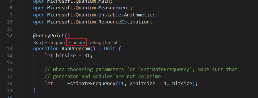
您可以選取一或多個 Qubit 參數 + 錯誤更正碼 類型,以估計資源。 在此範例中,選取 [qubit_gate_us_e3], 然後按兩下 [ 確定]。
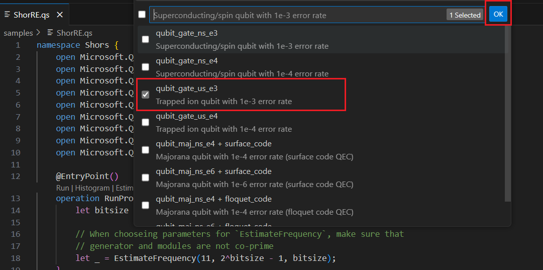
指定 [錯誤預算 ] 或接受預設值 0.001。 在此範例中,請保留預設值,然後按 Enter 鍵。
按 Enter 以根據檔名接受預設結果名稱,在此案例中為 ShorRE。
View the results
資源估算器會為相同的演算法提供多個估計值,每個估計值都會顯示量子位數目與運行時間之間的取捨。 瞭解運行時間和系統規模之間的取捨是資源估計的其中一個重要層面。
資源估計的結果會顯示在 [Q# 估計 ] 視窗中。
[ 結果] 索引 標籤會顯示資源估計的摘要。 按兩下 第一列旁的圖示,選取您想要顯示的數據行。 您可以從執行名稱、估計類型、量子位類型、qec 配置、錯誤預算、邏輯量子位、邏輯深度、程式代碼距離、T 狀態、T Factory、T Factory 分數、運行時間、rQOPS 和實體量子位中選取。
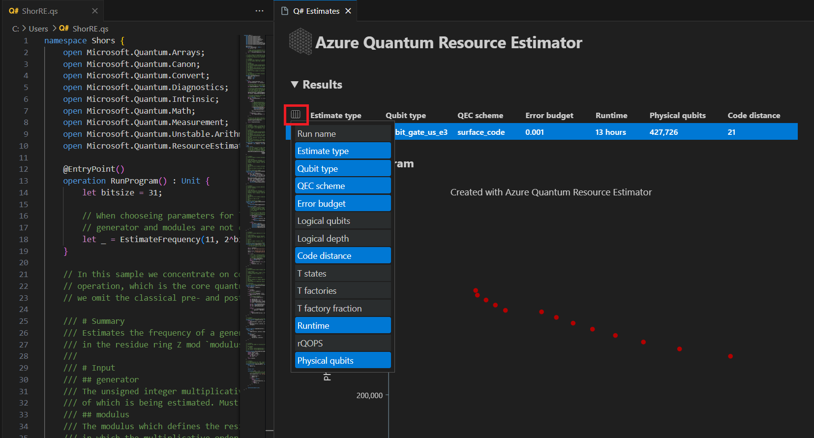
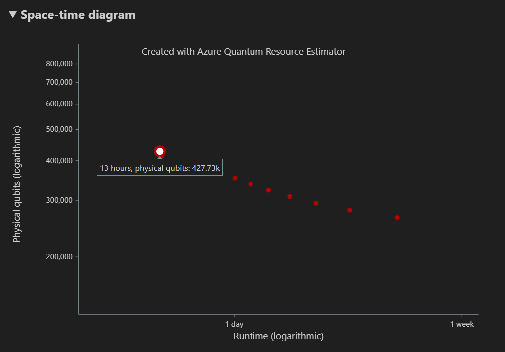
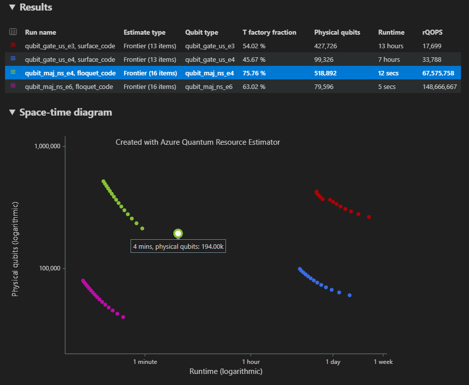
在結果數據表的 [估計類型 ] 數據行中,您可以看到演算法 的 {量子位數目、運行時間} 的最佳組合數目。 這些組合可以在空間時程圖表中看到。
空間時間圖表顯示實體量子位數目與演算法運行時間之間的取捨。 在此情況下,資源估算器會找出數千個可能組合的 13 種不同最佳組合。 您可以將滑鼠停留在每個 {number of qubits, runtime} 點上,以查看該時間點的資源估計詳細數據。
如需詳細資訊,請參閱 空間時程圖表。
注意
您必須 按兩下一個 空間時間點,也就是 {number of qubits, runtime} 組,以查看空間圖表,以及對應至該點的資源估計詳細數據。
[空間] 圖表顯示用於演算法的實體量子位分佈,以及對應至 {number of qubits, runtime} 配對的 T Factory。 例如,如果您在空間時間圖中選取最左邊的點,則執行演算法所需的實體量子位數目會427726,196686其中是演算法量子位,而其中 231040 是 T Factory 量子位。
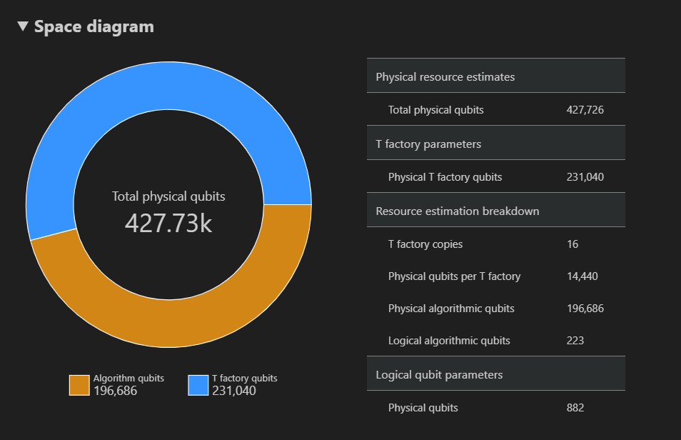
最後,[ 資源估計值 ] 索引卷標會顯示對應至 {number of qubits, runtime} 配對之 資源估算器的完整輸出數據清單。 您可以藉由折迭群組來檢查成本詳細資料,這些群組具有詳細資訊。 例如,選取空間時程圖表中最左邊的點,並折疊 邏輯量子位參數 群組。
邏輯量子位參數 值 QEC 配置 surface_code 程式碼距離 21 實際量子位元 882 邏輯週期時間 13 個錯誤 邏輯量子位錯誤率 3.00E-13 跨前置要素 0.03 錯誤修正臨界值 0.01 邏輯週期時間公式 (4 * + 2 * twoQubitGateTimeoneQubitMeasurementTime) *codeDistance實體量子位公式 2 * codeDistance*codeDistance提示
按兩下 [顯示詳細資料列 ] 以顯示報表資料之每個輸出的描述。
如需詳細資訊,請參閱 資源估算器的完整報表數據。
target變更參數
您可以使用其他量子位類型、錯誤修正碼和錯誤預算來估計相同 Q# 程式的成本。 選取 [ 檢視 -> 命令選擇區],然後輸入 Q#: Calculate Resource Estimates,以開啟 [資源估算器] 視窗。
選取任何其他組態,例如 Majorana 型量子位參數 qubit_maj_ns_e6。 接受預設的錯誤預算值或輸入新的值,然後按 Enter。 資源估算器會以新的 target 參數重新執行估計。
如需詳細資訊,請參閱資源估算器 的目標參數 。
執行多個參數位列態
Azure Quantum 資源估算器可以執行多個參數位列 target 態,並比較資源估計結果。
選取 [檢視 -> 命令選擇區],或按 Ctrl+Shift+P,然後輸入
Q#: Calculate Resource Estimates。選取 [qubit_gate_us_e3]、 [qubit_gate_us_e4]、 [qubit_maj_ns_e4 + floquet_code],然後 qubit_maj_ns_e6 + floquet_code,然後按兩下 [ 確定]。
接受預設錯誤預算值 0.001,然後按 Enter 鍵。
按 Enter 接受輸入檔,在此案例中為 ShorRE.qs。
如果是多個參數位列態,結果會顯示在 [ 結果 ] 索引卷標的不同數據列中。
空格時間圖表會顯示所有參數位列態的結果。 結果數據表的第一個數據行會顯示每個參數位態的圖例。 您可以將滑鼠停留在每個點上,以查看該點的資源估計詳細數據。
按兩下空間時程圖表 的 {number of qubits, runtime} 點 ,以顯示對應的空間圖表和報告數據。
VS Code 中 Jupyter Notebook 的必要條件
已安裝 Python 和 Pip 的 Python 環境。
最新版的 Visual Studio Code 或開啟 Web 上的 VS Code。
VS Code 已安裝 Azure Quantum Development Kit、 Python 和 Jupyter 擴充功能。
最新的 Azure Quantum
qsharp和qsharp-widgets套件。python -m pip install --upgrade qsharp qsharp-widgets
提示
您不需要有 Azure 帳戶才能執行本機資源估算器。
Create 量子演算法
在 VS Code 中,選取 [檢視>命令選擇區],然後選取 [Create:新增 Jupyter Notebook。
在右上方,VS Code 會偵測並顯示針對筆記本選取的 Python 版本和虛擬 Python 環境。 如果您有多個 Python 環境,您可能需要使用右上方的核心選擇器來選取核心。 如果未偵測到任何環境,請參閱 VS Code 中的 Jupyter Notebook 以 取得設定資訊。
在筆記本的第一個數據格中,匯入
qsharp套件。import qsharp新增數據格並複製下列程序代碼。
%%qsharp
open Microsoft.Quantum.Arrays;
open Microsoft.Quantum.Canon;
open Microsoft.Quantum.Convert;
open Microsoft.Quantum.Diagnostics;
open Microsoft.Quantum.Intrinsic;
open Microsoft.Quantum.Math;
open Microsoft.Quantum.Measurement;
open Microsoft.Quantum.Unstable.Arithmetic;
open Microsoft.Quantum.ResourceEstimation;

operation RunProgram() : Unit {
    let bitsize = 31;

    // When choosing parameters for `EstimateFrequency`, make sure that
    // generator and modules are not co-prime
    let _ = EstimateFrequency(11, 2^bitsize - 1, bitsize);
}


// In this sample we concentrate on costing the `EstimateFrequency`
// operation, which is the core quantum operation in Shors algorithm, and
// we omit the classical pre- and post-processing.

/// # Summary
/// Estimates the frequency of a generator
/// in the residue ring Z mod `modulus`.
///
/// # Input
/// ## generator
/// The unsigned integer multiplicative order (period)
/// of which is being estimated. Must be co-prime to `modulus`.
/// ## modulus
/// The modulus which defines the residue ring Z mod `modulus`
/// in which the multiplicative order of `generator` is being estimated.
/// ## bitsize
/// Number of bits needed to represent the modulus.
///
/// # Output
/// The numerator k of dyadic fraction k/2^bitsPrecision
/// approximating s/r.
operation EstimateFrequency(
    generator : Int,
    modulus : Int,
    bitsize : Int
)
: Int {
    mutable frequencyEstimate = 0;
    let bitsPrecision =  2 * bitsize + 1;

    // Allocate qubits for the superposition of eigenstates of
    // the oracle that is used in period finding.
    use eigenstateRegister = Qubit[bitsize];

    // Initialize eigenstateRegister to 1, which is a superposition of
    // the eigenstates we are estimating the phases of.
    // We first interpret the register as encoding an unsigned integer
    // in little endian encoding.
    ApplyXorInPlace(1, eigenstateRegister);
    let oracle = ApplyOrderFindingOracle(generator, modulus, _, _);

    // Use phase estimation with a semiclassical Fourier transform to
    // estimate the frequency.
    use c = Qubit();
    for idx in bitsPrecision - 1..-1..0 {
        within {
            H(c);
        } apply {
            // `BeginEstimateCaching` and `EndEstimateCaching` are the operations
            // exposed by Azure Quantum Resource Estimator. These will instruct
            // resource counting such that the if-block will be executed
            // only once, its resources will be cached, and appended in
            // every other iteration.
            if BeginEstimateCaching("ControlledOracle", SingleVariant()) {
                Controlled oracle([c], (1 <<< idx, eigenstateRegister));
                EndEstimateCaching();
            }
            R1Frac(frequencyEstimate, bitsPrecision - 1 - idx, c);
        }
        if MResetZ(c) == One {
            set frequencyEstimate += 1 <<< (bitsPrecision - 1 - idx);
        }
    }

    // Return all the qubits used for oracle eigenstate back to 0 state
    // using Microsoft.Quantum.Intrinsic.ResetAll.
    ResetAll(eigenstateRegister);

    return frequencyEstimate;
}

/// # Summary
/// Interprets `target` as encoding unsigned little-endian integer k
/// and performs transformation |k⟩ ↦ |gᵖ⋅k mod N ⟩ where
/// p is `power`, g is `generator` and N is `modulus`.
///
/// # Input
/// ## generator
/// The unsigned integer multiplicative order ( period )
/// of which is being estimated. Must be co-prime to `modulus`.
/// ## modulus
/// The modulus which defines the residue ring Z mod `modulus`
/// in which the multiplicative order of `generator` is being estimated.
/// ## power
/// Power of `generator` by which `target` is multiplied.
/// ## target
/// Register interpreted as little endian encoded which is multiplied by
/// given power of the generator. The multiplication is performed modulo
/// `modulus`.
internal operation ApplyOrderFindingOracle(
    generator : Int, modulus : Int, power : Int, target : Qubit[]
)
: Unit
is Adj + Ctl {
    // The oracle we use for order finding implements |x⟩ ↦ |x⋅a mod N⟩. We
    // also use `ExpModI` to compute a by which x must be multiplied. Also
    // note that we interpret target as unsigned integer in little-endian
    // encoding.
    ModularMultiplyByConstant(modulus,
                                ExpModI(generator, power, modulus),
                                target);
}

/// # Summary
/// Performs modular in-place multiplication by a classical constant.
///
/// # Description
/// Given the classical constants `c` and `modulus`, and an input
/// quantum register |𝑦⟩, this operation
/// computes `(c*x) % modulus` into |𝑦⟩.
///
/// # Input
/// ## modulus
/// Modulus to use for modular multiplication
/// ## c
/// Constant by which to multiply |𝑦⟩
/// ## y
/// Quantum register of target
internal operation ModularMultiplyByConstant(modulus : Int, c : Int, y : Qubit[])
: Unit is Adj + Ctl {
    use qs = Qubit[Length(y)];
    for (idx, yq) in Enumerated(y) {
        let shiftedC = (c <<< idx) % modulus;
        Controlled ModularAddConstant([yq], (modulus, shiftedC, qs));
    }
    ApplyToEachCA(SWAP, Zipped(y, qs));
    let invC = InverseModI(c, modulus);
    for (idx, yq) in Enumerated(y) {
        let shiftedC = (invC <<< idx) % modulus;
        Controlled ModularAddConstant([yq], (modulus, modulus - shiftedC, qs));
    }
}

/// # Summary
/// Performs modular in-place addition of a classical constant into a
/// quantum register.
///
/// # Description
/// Given the classical constants `c` and `modulus`, and an input
/// quantum register  |𝑦⟩, this operation
/// computes `(x+c) % modulus` into |𝑦⟩.
///
/// # Input
/// ## modulus
/// Modulus to use for modular addition
/// ## c
/// Constant to add to |𝑦⟩
/// ## y
/// Quantum register of target
internal operation ModularAddConstant(modulus : Int, c : Int, y : Qubit[])
: Unit is Adj + Ctl {
    body (...) {
        Controlled ModularAddConstant([], (modulus, c, y));
    }
    controlled (ctrls, ...) {
        // We apply a custom strategy to control this operation instead of
        // letting the compiler create the controlled variant for us in which
        // the `Controlled` functor would be distributed over each operation
        // in the body.
        //
        // Here we can use some scratch memory to save ensure that at most one
        // control qubit is used for costly operations such as `AddConstant`
        // and `CompareGreaterThenOrEqualConstant`.
        if Length(ctrls) >= 2 {
            use control = Qubit();
            within {
                Controlled X(ctrls, control);
            } apply {
                Controlled ModularAddConstant([control], (modulus, c, y));
            }
        } else {
            use carry = Qubit();
            Controlled AddConstant(ctrls, (c, y + [carry]));
            Controlled Adjoint AddConstant(ctrls, (modulus, y + [carry]));
            Controlled AddConstant([carry], (modulus, y));
            Controlled CompareGreaterThanOrEqualConstant(ctrls, (c, y, carry));
        }
    }
}

/// # Summary
/// Performs in-place addition of a constant into a quantum register.
///
/// # Description
/// Given a non-empty quantum register |𝑦⟩ of length 𝑛+1 and a positive
/// constant 𝑐 < 2ⁿ, computes |𝑦 + c⟩ into |𝑦⟩.
///
/// # Input
/// ## c
/// Constant number to add to |𝑦⟩.
/// ## y
/// Quantum register of second summand and target; must not be empty.
internal operation AddConstant(c : Int, y : Qubit[]) : Unit is Adj + Ctl {
    // We are using this version instead of the library version that is based
    // on Fourier angles to show an advantage of sparse simulation in this sample.

    let n = Length(y);
    Fact(n > 0, "Bit width must be at least 1");

    Fact(c >= 0, "constant must not be negative");
    Fact(c < 2 ^ n, $"constant must be smaller than {2L ^ n}");

    if c != 0 {
        // If c has j trailing zeroes than the j least significant bits
        // of y will not be affected by the addition and can therefore be
        // ignored by applying the addition only to the other qubits and
        // shifting c accordingly.
        let j = NTrailingZeroes(c);
        use x = Qubit[n - j];
        within {
            ApplyXorInPlace(c >>> j, x);
        } apply {
            IncByLE(x, y[j...]);
        }
    }
}

/// # Summary
/// Performs greater-than-or-equals comparison to a constant.
///
/// # Description
/// Toggles output qubit `target` if and only if input register `x`
/// is greater than or equal to `c`.
///
/// # Input
/// ## c
/// Constant value for comparison.
/// ## x
/// Quantum register to compare against.
/// ## target
/// Target qubit for comparison result.
///
/// # Reference
/// This construction is described in [Lemma 3, arXiv:2201.10200]
internal operation CompareGreaterThanOrEqualConstant(c : Int, x : Qubit[], target : Qubit)
: Unit is Adj+Ctl {
    let bitWidth = Length(x);

    if c == 0 {
        X(target);
    } elif c >= 2 ^ bitWidth {
        // do nothing
    } elif c == 2 ^ (bitWidth - 1) {
        ApplyLowTCNOT(Tail(x), target);
    } else {
        // normalize constant
        let l = NTrailingZeroes(c);

        let cNormalized = c >>> l;
        let xNormalized = x[l...];
        let bitWidthNormalized = Length(xNormalized);
        let gates = Rest(IntAsBoolArray(cNormalized, bitWidthNormalized));

        use qs = Qubit[bitWidthNormalized - 1];
        let cs1 = [Head(xNormalized)] + Most(qs);
        let cs2 = Rest(xNormalized);

        within {
            for i in IndexRange(gates) {
                (gates[i] ? ApplyAnd | ApplyOr)(cs1[i], cs2[i], qs[i]);
            }
        } apply {
            ApplyLowTCNOT(Tail(qs), target);
        }
    }
}

/// # Summary
/// Internal operation used in the implementation of GreaterThanOrEqualConstant.
internal operation ApplyOr(control1 : Qubit, control2 : Qubit, target : Qubit) : Unit is Adj {
    within {
        ApplyToEachA(X, [control1, control2]);
    } apply {
        ApplyAnd(control1, control2, target);
        X(target);
    }
}

internal operation ApplyAnd(control1 : Qubit, control2 : Qubit, target : Qubit)
: Unit is Adj {
    body (...) {
        CCNOT(control1, control2, target);
    }
    adjoint (...) {
        H(target);
        if (M(target) == One) {
            X(target);
            CZ(control1, control2);
        }
    }
}


/// # Summary
/// Returns the number of trailing zeroes of a number
///
/// ## Example
/// ```qsharp
/// let zeroes = NTrailingZeroes(21); // = NTrailingZeroes(0b1101) = 0
/// let zeroes = NTrailingZeroes(20); // = NTrailingZeroes(0b1100) = 2
/// ```
internal function NTrailingZeroes(number : Int) : Int {
    mutable nZeroes = 0;
    mutable copy = number;
    while (copy % 2 == 0) {
        set nZeroes += 1;
        set copy /= 2;
    }
    return nZeroes;
}

/// # Summary
/// An implementation for `CNOT` that when controlled using a single control uses
/// a helper qubit and uses `ApplyAnd` to reduce the T-count to 4 instead of 7.
internal operation ApplyLowTCNOT(a : Qubit, b : Qubit) : Unit is Adj+Ctl {
    body (...) {
        CNOT(a, b);
    }

    adjoint self;

    controlled (ctls, ...) {
        // In this application this operation is used in a way that
        // it is controlled by at most one qubit.
        Fact(Length(ctls) <= 1, "At most one control line allowed");

        if IsEmpty(ctls) {
            CNOT(a, b);
        } else {
            use q = Qubit();
            within {
                ApplyAnd(Head(ctls), a, q);
            } apply {
                CNOT(q, b);
            }
        }
    }

    controlled adjoint self;
}
估計量子演算法
現在,您會使用預設假設來估計作業的 RunProgram 實體資源。 新增數據格並複製下列程序代碼。
result = qsharp.estimate("RunProgram()")
result
函 qsharp.estimate 式會建立結果物件,可用來顯示具有整體實體資源計數的數據表。 您可以藉由折迭群組來檢查成本詳細資料,這些群組具有詳細資訊。 如需詳細資訊,請參閱 資源估算器的完整報表數據。
例如,折疊 邏輯量子位參數 群組,以查看程式代碼距離為 21,而實體量子位的數目為 882。
| 邏輯量子位參數 | 值 |
|---|---|
| QEC 配置 | surface_code |
| 程式碼距離 | 21 |
| 實際量子位元 | 882 |
| 邏輯週期時間 | 8 個 milisecs |
| 邏輯量子位錯誤率 | 3.00E-13 |
| 交叉前置要素 | 0.03 |
| 錯誤修正臨界值 | 0.01 |
| 邏輯週期時間公式 | (4 * twoQubitGateTime + 2 * oneQubitMeasurementTime) * codeDistance |
| 實體量子位公式 | 2 * codeDistance * codeDistance |
提示
如需更精簡版本的輸出資料表,您可以使用 result.summary。
空間圖
演算法和 T Factory 所使用的實體量子位分佈是可能會影響演算法設計的因素。 您可以使用 qsharp-widgets 套件將此分佈可視化,以進一步瞭解演算法的估計空間需求。
from qsharp-widgets import SpaceChart, EstimateDetails
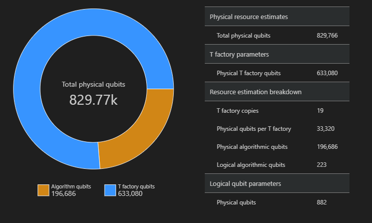
SpaceChart(result)
在此範例中,執行演算法所需的實體量子位數目是829766,其中196686為演算法量子位,其中 633080 是 T Factory 量子位。
變更預設值並估計演算法
提交計劃的資源估計要求時,您可以指定一些選擇性參數。 jobParams使用欄位來存取可傳遞至作業執行的所有target參數,並查看假設的預設值:
result['jobParams']
{'errorBudget': 0.001,
 'qecScheme': {'crossingPrefactor': 0.03,
  'errorCorrectionThreshold': 0.01,
  'logicalCycleTime': '(4 * twoQubitGateTime + 2 * oneQubitMeasurementTime) * codeDistance',
  'name': 'surface_code',
  'physicalQubitsPerLogicalQubit': '2 * codeDistance * codeDistance'},
 'qubitParams': {'instructionSet': 'GateBased',
  'name': 'qubit_gate_ns_e3',
  'oneQubitGateErrorRate': 0.001,
  'oneQubitGateTime': '50 ns',
  'oneQubitMeasurementErrorRate': 0.001,
  'oneQubitMeasurementTime': '100 ns',
  'tGateErrorRate': 0.001,
  'tGateTime': '50 ns',
  'twoQubitGateErrorRate': 0.001,
  'twoQubitGateTime': '50 ns'}}
您可以看到資源估算器會採用 qubit_gate_ns_e3 量子位模型、 surface_code 錯誤更正碼和 0.001 錯誤預算作為估計的預設值。
這些是 target 可自定義的參數:
errorBudget- 演算法的整體允許錯誤預算qecScheme- 量子錯誤修正 (QEC) 配置qubitParams- 實體量子位參數constraints- 元件層級的條件約束distillationUnitSpecifications- T Factory 擷取演算法的規格estimateType- 單一或新領域
如需詳細資訊,請參閱資源估算器 的目標參數 。
變更量子位模型
您可以使用Majorana型量子位參數、“ qubitParamsqubit_maj_ns_e6” 來估計相同演算法的成本。
result_maj = qsharp.estimate("RunProgram()", params={
                "qubitParams": {
                    "name": "qubit_maj_ns_e6"
                }})
EstimateDetails(result_maj)
變更量子錯誤修正配置
您可以在以 Majorana 為基礎的量子位參數上,使用已排開的 QEC 配置,重新執行資源估計作業。 qecScheme
result_maj = qsharp.estimate("RunProgram()", params={
                "qubitParams": {
                    "name": "qubit_maj_ns_e6"
                },
                "qecScheme": {
                    "name": "floquet_code"
                }})
EstimateDetails(result_maj)
變更錯誤預算
接下來,使用 errorBudget 10% 的 重新執行相同的量子線路。
result_maj = qsharp.estimate("RunProgram()", params={
                "qubitParams": {
                    "name": "qubit_maj_ns_e6"
                },
                "qecScheme": {
                    "name": "floquet_code"
                },
                "errorBudget": 0.1})
EstimateDetails(result_maj)
使用資源估算器批處理
Azure Quantum 資源估算器可讓您執行多個參陣列 target 態,並比較結果。 當您想要比較不同量子位模型、QEC 配置或錯誤預算的成本時,這非常有用。
您可以將參數清單 target 傳遞至
params函式的參數qsharp.estimate,以執行批次估計。 例如,使用預設參數和以 Majorana 為基礎的量子位參數搭配使用已排開的 QEC 配置來執行相同的演算法。result_batch = qsharp.estimate("RunProgram()", params= [{}, # Default parameters { "qubitParams": { "name": "qubit_maj_ns_e6" }, "qecScheme": { "name": "floquet_code" } }]) result_batch.summary_data_frame(labels=["Gate-based ns, 10⁻³", "Majorana ns, 10⁻⁶"])型號 邏輯量子位元 邏輯深度 T 狀態 程式碼距離 T Factory T Factory 分數 實際量子位元 rQOPS 實際執行時間 閘道型 ns, 10⁻³ 223 3.64M 4.70M 21 19 76.30 % 829.77k 26.55M 31 秒 Majorana ns, 10⁻⁶ 223 3.64M 4.70M 5 19 63.02 % 79.60k 148.67M 5 秒 您也可以使用
EstimatorParams類別建構估計參數清單。from qsharp.estimator import EstimatorParams, QubitParams, QECScheme, LogicalCounts labels = ["Gate-based µs, 10⁻³", "Gate-based µs, 10⁻⁴", "Gate-based ns, 10⁻³", "Gate-based ns, 10⁻⁴", "Majorana ns, 10⁻⁴", "Majorana ns, 10⁻⁶"] params = EstimatorParams(num_items=6) params.error_budget = 0.333 params.items[0].qubit_params.name = QubitParams.GATE_US_E3 params.items[1].qubit_params.name = QubitParams.GATE_US_E4 params.items[2].qubit_params.name = QubitParams.GATE_NS_E3 params.items[3].qubit_params.name = QubitParams.GATE_NS_E4 params.items[4].qubit_params.name = QubitParams.MAJ_NS_E4 params.items[4].qec_scheme.name = QECScheme.FLOQUET_CODE params.items[5].qubit_params.name = QubitParams.MAJ_NS_E6 params.items[5].qec_scheme.name = QECScheme.FLOQUET_CODEqsharp.estimate("RunProgram()", params=params).summary_data_frame(labels=labels)型號 邏輯量子位元 邏輯深度 T 狀態 程式碼距離 T Factory T Factory 分數 實際量子位元 rQOPS 實際執行時間 閘道型 µs, 10⁻³ 223 3.64M 4.70M 17 13 40.54 % 216.77k 21.86k 10 個小時 閘道型 µs, 10⁻⁴ 223 3.64M 4.70M 9 14 43.17 % 63.57k 41.30k 5 個小時 閘道型 ns, 10⁻³ 223 3.64M 4.70M 17 16 69.08 % 416.89k 32.79M 25 秒 閘道型 ns, 10⁻⁴ 223 3.64M 4.70M 9 14 43.17 % 63.57k 61.94M 13 秒 Majorana ns, 10⁻⁴ 223 3.64M 4.70M 9 19 82.75 % 501.48k 82.59M 10 秒 Majorana ns, 10⁻⁶ 223 3.64M 4.70M 5 13 31.47 % 42.96k 148.67M 5 秒
執行 Pareto 新領域估計
估計演算法的資源時,請務必考慮實體量子位數目與演算法運行時間之間的取捨。 您可以考慮盡可能配置多個實體量子位,以減少演算法的運行時間。 不過,實體量子位的數目受限於量子硬體中可用的實體量子位數目。
Pareto 新領域估計會提供相同演算法的多個估計值,每個演算法在量子位數目與運行時間之間都有取捨。
若要使用 Pareto 前項估計來執行資源估算器,您必須將 參數指定
"estimateType"target 為"frontier"。 例如,使用以 Majorana 為基礎的量子位參數,使用 Pareto 新領域估計,以表面程式代碼執行相同的演算法。result = qsharp.estimate("RunProgram()", params= {"qubitParams": { "name": "qubit_maj_ns_e4" }, "qecScheme": { "name": "surface_code" }, "estimateType": "frontier", # frontier estimation } )您可以使用 函
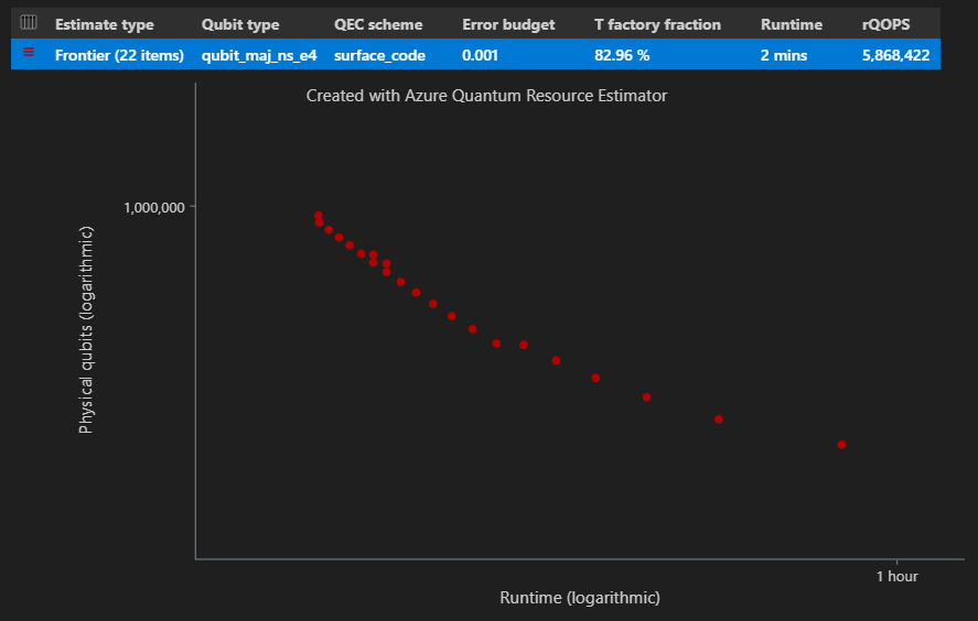
EstimatesOverview式來顯示具有整體實體資源計數的數據表。 按兩下第一列旁的圖示,選取您想要顯示的數據行。 您可以從執行名稱、估計類型、量子位類型、qec 配置、錯誤預算、邏輯量子位、邏輯深度、程式代碼距離、T 狀態、T Factory、T Factory 分數、運行時間、rQOPS 和實體量子位中選取。from qsharp_widgets import EstimatesOverview EstimatesOverview(result)
在結果數據表的 [ 估計類型 ] 數據行中,您可以看到演算法的 {量子位數目、運行時間} 的不同組合數目。 在此情況下,資源估算器會找出數千個可能組合的 22 個不同最佳組合。
空間時程圖表
函 EstimatesOverview 式也會顯示資源估算器的空間 時程圖表 。
空間時間圖表會顯示每個 {qubits, runtime} 配對之演演算法的實體量子位數目和運行時間。 您可以將滑鼠停留在每個點上,以查看該點的資源估計詳細數據。
使用 Pareto 新領域估計進行批處理
若要估計和比較多個參數位列 target 態與新進階估計,請將 新增
"estimateType": "frontier",至參數。result = qsharp.estimate( "RunProgram()", [ { "qubitParams": { "name": "qubit_maj_ns_e4" }, "qecScheme": { "name": "surface_code" }, "estimateType": "frontier", # Pareto frontier estimation }, { "qubitParams": { "name": "qubit_maj_ns_e6" }, "qecScheme": { "name": "floquet_code" }, "estimateType": "frontier", # Pareto frontier estimation }, ] ) EstimatesOverview(result, colors=["#1f77b4", "#ff7f0e"], runNames=["e4 Surface Code", "e6 Floquet Code"])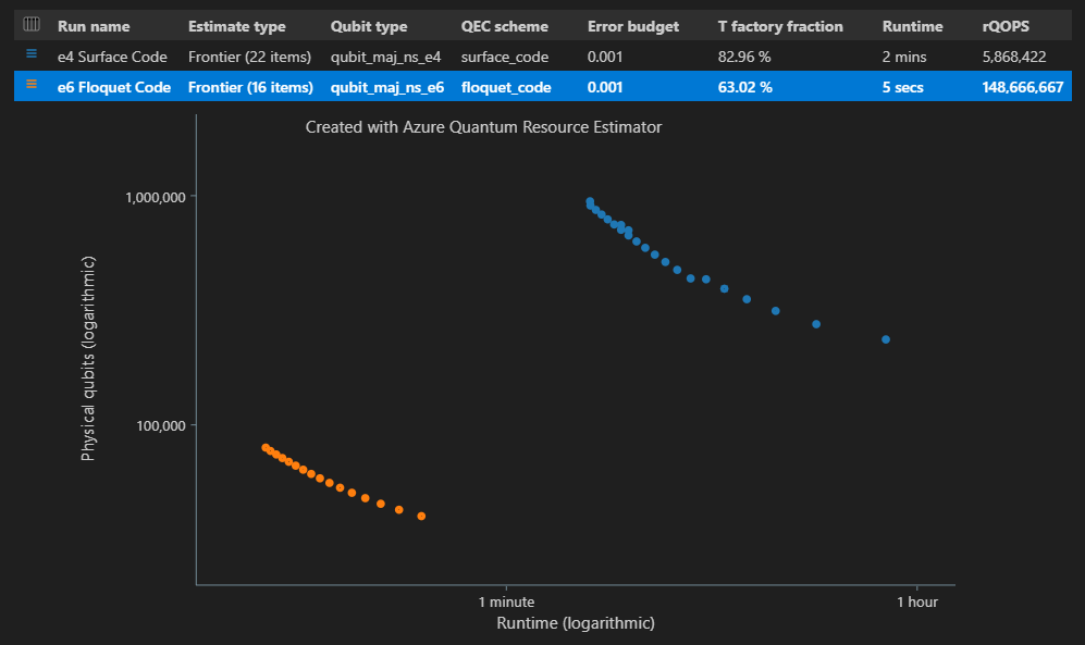
注意
您可以使用 函式來定義量子位時間圖表
EstimatesOverview的色彩和執行名稱。使用 Pareto 新進階估計執行多個 target 參數位態時,您可以看到空間時程圖表中特定時間點的資源估計值,也就是每個 {量子位數目、運行時間} 組。 例如,下列程式代碼會顯示第二個 (估計索引=0) 執行的估計詳細數據使用量,以及第四個 (點索引=3) 最短運行時間。
EstimateDetails(result[1], 4)您也可以查看空間時間圖的特定時間點的空間圖表。 例如,下列程式代碼顯示第一次執行組合的空間圖表, (估計 index=0) ,以及第三個最短運行時間 (點索引=2) 。
SpaceChart(result[0], 2)
Qiskit 的必要條件
- 具備有效訂用帳戶的 Azure 帳戶。 如果您沒有 Azure 帳戶,請免費註冊並註冊 隨用隨付訂用帳戶。
- Azure Quantum 工作區。 如需詳細資訊,請參閱建立 Azure Quantum 工作區。
在您的工作區中啟用 Azure Quantum 資源估算器target
資源估算器是 target Microsoft Quantum Computing 提供者的。 如果您在資源估算器發行后建立了工作區,Microsoft Quantum Computing 提供者會自動新增至您的工作區。
如果您使用 現有的 Azure Quantum 工作區:
- 在 Azure 入口網站中開啟工作區。
- 在左側面板的 [ 作業] 下,選取 [ 提供者]。
- 選取 [+ 新增提供者]。
- 針對 Microsoft Quantum Computing 選取 [+ 新增]。
- 選取 [學習 & 開發 ],然後選取 [ 新增]。
在工作區中建立新的筆記本
- 登入 Azure 入口網站,並選取您的 Azure Quantum 工作區。
- 在 [作業] 底下,選取 [筆記本]
- 按兩下 [我的筆記本] ,然後按兩下 [ 新增]
- 在 [核心類型]中,選取 [IPython]。
- 輸入檔案的名稱,然後按兩下 [Create 檔案]。
當您的新筆記本開啟時,會根據您的訂用帳戶和工作區資訊自動建立第一個儲存格的程式碼。
from azure.quantum import Workspace
workspace = Workspace (
    resource_id = "", # Your resource_id
    location = ""  # Your workspace location (for example, "westus")
)
注意
除非另有說明,否則建立儲存格時,您應該依序執行每個儲存格,避免任何編譯問題。
請按一下儲存格左側的三角形「播放」圖示,執行程式碼。
載入必要的匯入
首先,您必須從 azure-quantum 和 qiskit匯入其他模組。
按一下 [+ 程式碼] 新增儲存格,然後新增並執行下列程式碼:
from azure.quantum.qiskit import AzureQuantumProvider
from qiskit import QuantumCircuit, transpile
from qiskit.circuit.library import RGQFTMultiplier
連線 Azure Quantum 服務
接下來,使用workspace上一個單元格中的 物件來建立 AzureQuantumProvider 物件,以連線到您的 Azure Quantum 工作區。 您可以建立後端實例,並將資源估算器設定為 。target
provider = AzureQuantumProvider(workspace)
backend = provider.get_backend('microsoft.estimator')
Create 量子演算法
在此範例中,您會根據 Ruiz-Perez 和 Garcia-Escartin (arXiv:1411.5949) 中呈現的建構來建立乘數的量子電路,其會使用 Quantum Fourier Transform 來實作算術。
您可以藉由變更 bitwidth 變數來調整乘數的大小。 線路產生會包裝在可透過 bitwidth 乘數值呼叫的函式中。 作業會有兩個輸入緩存器,每個輸入緩存器的大小都是指定的 bitwidth,以及一個輸出緩存器,其大小為指定 bitwidth的大小兩倍。 函式也會列印直接從量子線路擷取之乘數的一些邏輯資源計數。
def create_algorithm(bitwidth):
    print(f"[INFO] Create a QFT-based multiplier with bitwidth {bitwidth}")

    # Print a warning for large bitwidths that will require some time to generate and
    # transpile the circuit.
    if bitwidth > 18:
        print(f"[WARN] It will take more than one minute generate a quantum circuit with a bitwidth larger than 18")

    circ = RGQFTMultiplier(num_state_qubits=bitwidth, num_result_qubits=2 * bitwidth)

    # One could further reduce the resource estimates by increasing the optimization_level,
    # however, this will also increase the runtime to construct the algorithm.  Note, that
    # it does not affect the runtime for resource estimation.
    print(f"[INFO] Decompose circuit into intrinsic quantum operations")

    circ = transpile(circ, basis_gates=SUPPORTED_INSTRUCTIONS, optimization_level=0)

    # print some statistics
    print(f"[INFO]   qubit count: {circ.num_qubits}")
    print("[INFO]   gate counts")
    for gate, count in circ.count_ops().items():
        print(f"[INFO]   - {gate}: {count}")

    return circ
注意
您可以針對沒有 T 狀態但至少有一個度量的演算法提交實體資源估計作業。
估計量子演算法
使用函式 Create 演算法create_algorithm的實例。 您可以藉由變更 bitwidth 變數來調整乘數的大小。
bitwidth = 4

circ = create_algorithm(bitwidth)
使用預設假設來估計此作業的實體資源。 您可以使用 方法將線路提交至資源估算器後端 run ,然後執行 job.result() 以等候作業完成並傳回結果。
job = backend.run(circ)
result = job.result()
result
這會建立顯示整體實體資源計數的數據表。 您可以藉由折迭群組來檢查成本詳細資料,這些群組具有詳細資訊。
提示
如需更精簡版本的輸出資料表,您可以使用 result.summary。
例如,如果您折疊 邏輯量子位參數 群組,您可以更輕鬆地看到錯誤更正碼距離為 15。
| 邏輯量子位參數 | 值 |
|---|---|
| QEC 配置 | surface_code |
| 程式碼距離 | 15 |
| 實際量子位元 | 450 |
| 邏輯週期時間 | 6us |
| 邏輯量子位錯誤率 | 3.00E-10 |
| 交叉前置要素 | 0.03 |
| 錯誤修正臨界值 | 0.01 |
| 邏輯週期時間公式 | (4 * twoQubitGateTime + 2 * oneQubitMeasurementTime) * codeDistance |
| 實體量子位公式 | 2 * codeDistance * codeDistance |
在 [實體量子位參數 ] 群組中,您可以看到針對此估計所假設的實體量子位屬性。 例如,分別假設執行單一量子位測量和單一量子位閘道的時間是 100 奈秒和 50 奈秒。
提示
您也可以使用 result.data () 方法,以 Python 字典的形式存取資源估算器的輸出。
如需詳細資訊,請參閱資源估算器 的完整輸出數據清單 。
空間圖
演算法和 T Factory 所使用的實體量子位分佈是可能會影響演算法設計的因素。 您可以將此分佈可視化,以進一步瞭解演算法的估計空間需求。
result.diagram.space
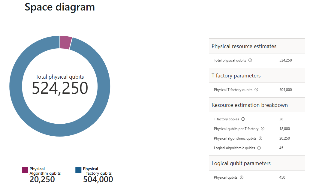
空間圖顯示演算法量子位和 T Factory 量子位的比例。 請注意,T Factory 複本數目 28 會參與 T Factory 的實體量子位數目,因為 $\text{T factoryies} \cdot \text{physical qubit per T factory}= 28 \cdot 18,000 = 504,000$。
如需詳細資訊,請參閱 T Factory 實體估計。
變更預設值並估計演算法
提交計劃的資源估計要求時,您可以指定一些選擇性參數。 jobParams使用欄位來存取可傳遞至作業執行的所有值,並查看假設的預設值:
result.data()["jobParams"]
{'errorBudget': 0.001,
 'qecScheme': {'crossingPrefactor': 0.03,
  'errorCorrectionThreshold': 0.01,
  'logicalCycleTime': '(4 * twoQubitGateTime + 2 * oneQubitMeasurementTime) * codeDistance',
  'name': 'surface_code',
  'physicalQubitsPerLogicalQubit': '2 * codeDistance * codeDistance'},
 'qubitParams': {'instructionSet': 'GateBased',
  'name': 'qubit_gate_ns_e3',
  'oneQubitGateErrorRate': 0.001,
  'oneQubitGateTime': '50 ns',
  'oneQubitMeasurementErrorRate': 0.001,
  'oneQubitMeasurementTime': '100 ns',
  'tGateErrorRate': 0.001,
  'tGateTime': '50 ns',
  'twoQubitGateErrorRate': 0.001,
  'twoQubitGateTime': '50 ns'}}
這些是 target 可自定義的參數:
errorBudget- 整體允許的錯誤預算qecScheme- 量子錯誤修正 (QEC) 配置qubitParams- 實體量子位參數constraints- 元件層級的條件約束distillationUnitSpecifications- T Factory 擷取演算法的規格
如需詳細資訊,請參閱資源估算器 的目標參數 。
變更量子位模型
接下來,使用Majorana型量子位參數來估計相同演算法的成本 qubit_maj_ns_e6
job = backend.run(circ,
    qubitParams={
        "name": "qubit_maj_ns_e6"
    })
result = job.result()
result
您可以透過程式設計方式檢查實體計數。 例如,您可以探索建立以執行演算法之 T Factory 的詳細數據。
result.data()["tfactory"]
{'eccDistancePerRound': [1, 1, 5],
 'logicalErrorRate': 1.6833177305222897e-10,
 'moduleNamePerRound': ['15-to-1 space efficient physical',
  '15-to-1 RM prep physical',
  '15-to-1 RM prep logical'],
 'numInputTstates': 20520,
 'numModulesPerRound': [1368, 20, 1],
 'numRounds': 3,
 'numTstates': 1,
 'physicalQubits': 16416,
 'physicalQubitsPerRound': [12, 31, 1550],
 'runtime': 116900.0,
 'runtimePerRound': [4500.0, 2400.0, 110000.0]}
注意
根據預設,運行時間會顯示為 nanoseconds。
您可以使用此資料來產生 T Factory 如何產生必要 T 狀態的一些說明。
data = result.data()
tfactory = data["tfactory"]
breakdown = data["physicalCounts"]["breakdown"]
producedTstates = breakdown["numTfactories"] * breakdown["numTfactoryRuns"] * tfactory["numTstates"]

print(f"""A single T factory produces {tfactory["logicalErrorRate"]:.2e} T states with an error rate of (required T state error rate is {breakdown["requiredLogicalTstateErrorRate"]:.2e}).""")
print(f"""{breakdown["numTfactories"]} copie(s) of a T factory are executed {breakdown["numTfactoryRuns"]} time(s) to produce {producedTstates} T states ({breakdown["numTstates"]} are required by the algorithm).""")
print(f"""A single T factory is composed of {tfactory["numRounds"]} rounds of distillation:""")
for round in range(tfactory["numRounds"]):
    print(f"""- {tfactory["numModulesPerRound"][round]} {tfactory["moduleNamePerRound"][round]} unit(s)""")
A single T factory produces 1.68e-10 T states with an error rate of (required T state error rate is 2.77e-08).
23 copies of a T factory are executed 523 time(s) to produce 12029 T states (12017 are required by the algorithm).
A single T factory is composed of 3 rounds of distillation:
- 1368 15-to-1 space efficient physical unit(s)
- 20 15-to-1 RM prep physical unit(s)
- 1 15-to-1 RM prep logical unit(s)
變更量子錯誤修正配置
現在,在以 Majorana 為基礎的量子位參數上,使用已排開的 QEC 配置重新執行相同範例的資源估計作業。 qecScheme
job = backend.run(circ,
    qubitParams={
        "name": "qubit_maj_ns_e6"
    },
    qecScheme={
        "name": "floquet_code"
    })
result_maj_floquet = job.result()
result_maj_floquet
變更錯誤預算
讓我們以 10% 的 重新 errorBudget 執行相同的量子線路。
job = backend.run(circ,
    qubitParams={
        "name": "qubit_maj_ns_e6"
    },
    qecScheme={
        "name": "floquet_code"
    },
    errorBudget=0.1)
result_maj_floquet_e1 = job.result()
result_maj_floquet_e1
注意
如果您在使用資源估算器時遇到任何問題,請參閱 疑難解答頁面,或連絡 AzureQuantumInfo@microsoft.com。
下一步
意見反應
即將登場:在 2024 年,我們將逐步淘汰 GitHub 問題作為內容的意見反應機制,並將它取代為新的意見反應系統。 如需詳細資訊,請參閱:https://aka.ms/ContentUserFeedback。
提交並檢視相關的意見反應