教學課程：使用 Apache Spark MLlib 和 Azure Synapse Analytics 來建置機器學習應用程式

發行項
02/29/2024

在本文中，您將了解如何使用 Apache Spark MLlib 建立機器學習應用程式，在 Azure 開放資料集上進行簡單預測性分析。 Spark 提供內建的機器學習程式庫。這個範例會透過羅吉斯迴歸使用「分類」。

SparkML 和 MLlib 是核心 Spark 程式庫，提供許多可用於機器學習工作的公用程式，包括具有下列用途的公用程式：

分類
迴歸
叢集
主題模型化
奇異值分解 (SVD) 和主體元件分析 (PCA)
假設測試和計算範例統計資料

了解分類和羅吉斯迴歸

分類是常見的機器學習工作，是指將輸入資料依類別排序的程序。這是以分類演算法指出如何為您所提供的輸入資料指派「標籤」的作業。例如，試想某個機器學習演算法以股市資訊作為輸入，並且將股票分成兩個類別：該賣的股票和該留的股票。

「羅吉斯迴歸」是您可以用於分類的演算法。 Spark 的羅吉斯迴歸 API 可用於二元分類，或用來將輸入資料歸類到兩個群組之一。如需羅吉斯迴歸的詳細資訊，請參閱 Wikipedia。

總之，羅吉斯迴歸的程序會產生一個羅吉斯函數，此函數可用來預測輸入向量可能屬於哪一個群組的機率。

紐約市計程車資料的預測分析範例

在此範例中，您會使用 Spark 對紐約的計程車行程小費資料執行一些預測分析。您可以透過 Azure 開放資料集取得資料。此資料集的子集包含黃色計程車行程的相關資訊，包括每個行程的相關資訊、開始和結束時間及位置、成本和其他有趣的屬性。

重要

從其儲存體位置提取此資料可能會產生額外費用。

在下列步驟中，您會開發模型來預測特定行程是否包含小費。

建立 Apache Spark 機器學習模型

使用 PySpark 核心建立筆記本。如需相關指示，請參閱建立筆記本。

匯入此應用程式所需的類型。複製以下程式碼並貼入空白儲存格，然後按下 Shift+Enter 鍵。或使用程式碼左邊的藍色播放圖示來執行儲存格。

import matplotlib.pyplot as plt
from datetime import datetime
from dateutil import parser
from pyspark.sql.functions import unix_timestamp, date_format, col, when
from pyspark.ml import Pipeline
from pyspark.ml import PipelineModel
from pyspark.ml.feature import RFormula
from pyspark.ml.feature import OneHotEncoder, StringIndexer, VectorIndexer
from pyspark.ml.classification import LogisticRegression
from pyspark.mllib.evaluation import BinaryClassificationMetrics
from pyspark.ml.evaluation import BinaryClassificationEvaluator

由於使用 PySpark 核心，因此不需要明確建立任何內容。當您執行第一個程式碼儲存格時，系統會自動為您建立 Spark 內容。

建構輸入資料框架

因為未經處理的資料採用 Parquet 格式，所以您可以使用 Spark 內容，直接將檔案當作資料框架提取至記憶體中。雖然下列步驟中的程式碼使用預設選項，但是您可以視需要強制對應資料類型和其他結構描述屬性。

執行下列幾行，將程式碼貼至新的儲存格來建立 Spark 資料框架。這個步驟會透過開放資料集 API 來擷取資料。提取所有資料會產生大約 15 億個資料列。

根據您的無伺服器 Apache Spark 集區大小，未經處理資料可能太大，或花費太多時間來操作。您可以將此資料篩選成較小的項目。下列程式碼範例會使用 start_date 和 end_date 來套用篩選器，以傳回單一月份的資料。
```
from azureml.opendatasets import NycTlcYellow

from datetime import datetime
from dateutil import parser

end_date = parser.parse('2018-05-08 00:00:00')
start_date = parser.parse('2018-05-01 00:00:00')

nyc_tlc = NycTlcYellow(start_date=start_date, end_date=end_date)
filtered_df = spark.createDataFrame(nyc_tlc.to_pandas_dataframe())
```
從統計觀點來看，簡單篩選的缺點是可能會導致資料偏差。另一種方法是使用 Spark 內建的取樣。

如果在上述程式碼之後套用，下列程式碼會將資料集縮減為大約 2000 個資料列。您可以使用此取樣步驟來取代簡單篩選，或與簡單篩選搭配使用。
```
# To make development easier, faster, and less expensive, downsample for now
sampled_taxi_df = filtered_df.sample(True, 0.001, seed=1234)
```
您現在可以查看資料，以查看已讀取的內容。根據資料集的大小而定，通常最好是使用子集來檢閱資料，而不是使用完整集合。

下列程式碼提供兩種方式來檢視資料。第一種方式是基本。第二種方式提供更豐富的格線體驗，以及以圖形方式視覺化資料的功能。
```
#sampled_taxi_df.show(5)
display(sampled_taxi_df)
```
根據所產生的資料集大小，以及您實驗或執行筆記本多次的需求而定，您可能想要在工作區中的本機快取資料集。有三種方式可執行明確的快取：
- 以檔案的形式將資料框架儲存在本機。
- 將資料框架儲存為暫存資料表或檢視。
- 將資料框架儲存為永久資料表。

下列程式碼範例包含這些方法的前兩個。

建立暫存資料表或檢視會提供不同的資料存取路徑，但是只會持續到 Spark 執行個體工作階段的持續時間。

sampled_taxi_df.createOrReplaceTempView("nytaxi")

準備資料

未經處理格式的資料通常不適合直接傳遞至模型。您必須對資料執行一系列的動作，才能使其進入模型可以取用的狀態。

在下列程式碼中，您會執行四個類別的作業：

透過篩選移除極端值或不正確的值。
移除不需要的資料行。
建立衍生自未經處理資料的新資料行，讓模型運作更有效率。這項作業有時稱為特徵化。
加上標籤。因為您正在進行二元分類 (指定行程是否有小費)，因此需要將小費金額轉換成 0 或 1 的值。

taxi_df = sampled_taxi_df.select('totalAmount', 'fareAmount', 'tipAmount', 'paymentType', 'rateCodeId', 'passengerCount'\
                                , 'tripDistance', 'tpepPickupDateTime', 'tpepDropoffDateTime'\
                                , date_format('tpepPickupDateTime', 'hh').alias('pickupHour')\
                                , date_format('tpepPickupDateTime', 'EEEE').alias('weekdayString')\
                                , (unix_timestamp(col('tpepDropoffDateTime')) - unix_timestamp(col('tpepPickupDateTime'))).alias('tripTimeSecs')\
                                , (when(col('tipAmount') > 0, 1).otherwise(0)).alias('tipped')
                                )\
                        .filter((sampled_taxi_df.passengerCount > 0) & (sampled_taxi_df.passengerCount < 8)\
                                & (sampled_taxi_df.tipAmount >= 0) & (sampled_taxi_df.tipAmount <= 25)\
                                & (sampled_taxi_df.fareAmount >= 1) & (sampled_taxi_df.fareAmount <= 250)\
                                & (sampled_taxi_df.tipAmount < sampled_taxi_df.fareAmount)\
                                & (sampled_taxi_df.tripDistance > 0) & (sampled_taxi_df.tripDistance <= 100)\
                                & (sampled_taxi_df.rateCodeId <= 5)
                                & (sampled_taxi_df.paymentType.isin({"1", "2"}))
                                )

接著會對資料進行第二次傳遞，以新增最終特性。

taxi_featurised_df = taxi_df.select('totalAmount', 'fareAmount', 'tipAmount', 'paymentType', 'passengerCount'\
                                                , 'tripDistance', 'weekdayString', 'pickupHour','tripTimeSecs','tipped'\
                                                , when((taxi_df.pickupHour <= 6) | (taxi_df.pickupHour >= 20),"Night")\
                                                .when((taxi_df.pickupHour >= 7) & (taxi_df.pickupHour <= 10), "AMRush")\
                                                .when((taxi_df.pickupHour >= 11) & (taxi_df.pickupHour <= 15), "Afternoon")\
                                                .when((taxi_df.pickupHour >= 16) & (taxi_df.pickupHour <= 19), "PMRush")\
                                                .otherwise(0).alias('trafficTimeBins')
                                              )\
                                       .filter((taxi_df.tripTimeSecs >= 30) & (taxi_df.tripTimeSecs <= 7200))

建立羅吉斯迴歸模型

最後一項工作，是將加上標籤的資料轉換成可透過羅吉斯迴歸進行分析的格式。羅吉斯迴歸演算法的輸入必須是一組「標籤/特性向量配對」，其中「特性向量」是代表輸入點的數字向量。

因此，您需要將類別資料行轉換成數字。具體而言，您需要將 trafficTimeBins 和 weekdayString 資料行轉換成整數表示。有多種方法可以執行轉換。下列範例會採用常見的 OneHotEncoder 方法。

# Because the sample uses an algorithm that works only with numeric features, convert them so they can be consumed
sI1 = StringIndexer(inputCol="trafficTimeBins", outputCol="trafficTimeBinsIndex")
en1 = OneHotEncoder(dropLast=False, inputCol="trafficTimeBinsIndex", outputCol="trafficTimeBinsVec")
sI2 = StringIndexer(inputCol="weekdayString", outputCol="weekdayIndex")
en2 = OneHotEncoder(dropLast=False, inputCol="weekdayIndex", outputCol="weekdayVec")

# Create a new DataFrame that has had the encodings applied
encoded_final_df = Pipeline(stages=[sI1, en1, sI2, en2]).fit(taxi_featurised_df).transform(taxi_featurised_df)

此動作會產生新的資料框架，其中包含正確格式的所有資料行來定型模型。

定型羅吉斯迴歸模型

第一個工作是將資料集分割成定型集和測試或驗證集。此處的分割是任意的。使用不同的分割設定進行實驗，以查看是否會影響模型。

# Decide on the split between training and testing data from the DataFrame
trainingFraction = 0.7
testingFraction = (1-trainingFraction)
seed = 1234

# Split the DataFrame into test and training DataFrames
train_data_df, test_data_df = encoded_final_df.randomSplit([trainingFraction, testingFraction], seed=seed)

現在有兩個資料框架，下一個工作是建立模型公式，然後針對定型資料框架執行。接著，您可以針對測試資料框架進行驗證。使用不同版本的模型公式來進行實驗，以查看不同組合的影響。

注意

若要儲存模型，請將儲存體 Blob 資料參與者角色指派給 Azure SQL Database 伺服器資源範圍。如需詳細步驟，請參閱使用 Azure 入口網站指派 Azure 角色。僅有具備擁有者權限的成員才能執行此步驟。

## Create a new logistic regression object for the model
logReg = LogisticRegression(maxIter=10, regParam=0.3, labelCol = 'tipped')

## The formula for the model
classFormula = RFormula(formula="tipped ~ pickupHour + weekdayVec + passengerCount + tripTimeSecs + tripDistance + fareAmount + paymentType+ trafficTimeBinsVec")

## Undertake training and create a logistic regression model
lrModel = Pipeline(stages=[classFormula, logReg]).fit(train_data_df)

## Saving the model is optional, but it's another form of inter-session cache
datestamp = datetime.now().strftime('%m-%d-%Y-%s')
fileName = "lrModel_" + datestamp
logRegDirfilename = fileName
lrModel.save(logRegDirfilename)

## Predict tip 1/0 (yes/no) on the test dataset; evaluation using area under ROC
predictions = lrModel.transform(test_data_df)
predictionAndLabels = predictions.select("label","prediction").rdd
metrics = BinaryClassificationMetrics(predictionAndLabels)
print("Area under ROC = %s" % metrics.areaUnderROC)

此儲存格的輸出為：

Area under ROC = 0.9779470729751403

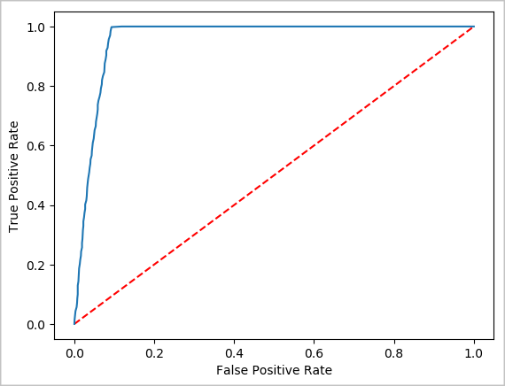
建立預測的視覺表示法

您現在可以建構最終的視覺效果，以利研判此測試的結果。 ROC 曲線是檢閱結果的一種方式。

## Plot the ROC curve; no need for pandas, because this uses the modelSummary object
modelSummary = lrModel.stages[-1].summary

plt.plot([0, 1], [0, 1], 'r--')
plt.plot(modelSummary.roc.select('FPR').collect(),
         modelSummary.roc.select('TPR').collect())
plt.xlabel('False Positive Rate')
plt.ylabel('True Positive Rate')
plt.show()

此圖表顯示小費模型中羅吉斯迴歸的 ROC 曲線。

關閉 Spark 執行個體

當您完成執行應用程式之後，請藉由關閉索引標籤，或從筆記本底部的狀態面板中選取 [結束工作階段]，關閉筆記本以釋放資源。

另請參閱

概觀：Azure Synapse Analytics 上的 Apache Spark

後續步驟

注意

某些 Apache Spark 官方文件會依賴使用 Spark 主控台，但 Azure Synapse Analytics 中的 Apache Spark 不提供這項功能。請改用 Notebook 或 IntelliJ 體驗。