Query processing architecture guide

Applies to: SQL Server Azure SQL Database Azure SQL Managed Instance SQL database in Microsoft Fabric

The SQL Server Database Engine processes queries on various data storage architectures such as local tables, partitioned tables, and tables distributed across multiple servers. The following sections cover how the Database Engine processes queries and optimizes query reuse through execution plan caching.

The code samples in this article use the AdventureWorks2025, AdventureWorksDW2025, or AdventureWorksLT2025 sample database, which you can download from the Azure Data SQL Samples Repository GitHub repository.

Execution modes

The SQL Server Database Engine can process Transact-SQL (T-SQL) statements using two distinct processing modes:

• Row mode execution
• Batch mode execution

Row mode execution

Row mode execution is a query processing method used with rowstore tables and indexes, where data is stored in row format. When a query is executed and accesses data in rowstore tables and indexes, the execution tree operators and child operators read each required row, across all the columns specified in the object schema. From each row that is read, the Database Engine then retrieves the columns that are required for the result set, as referenced by a SELECT statement, JOIN predicate, or filter predicate.

Note

Row mode execution is very efficient for OLTP scenarios, but it can be less efficient when scanning large amounts of data, for example in Data Warehousing scenarios.

Batch mode execution

Batch mode execution is a query processing method that processes multiple rows together (hence the term batch). Each column within a batch is stored as a vector in a separate area of memory, so batch mode processing is vector-based. Batch mode processing also uses algorithms that are optimized for the advanced instruction sets and increased memory throughput in modern processors.

Batch mode execution was originally integrated and optimized around the columnstore storage format. Starting with SQL Server 2019 (15.x) and in Azure SQL Database, batch mode execution doesn't require columnstore indexes. For more information, see Batch mode on rowstore.

Batch mode processing operates on compressed data when possible, and it eliminates the exchange operator that row mode execution uses. The result is better parallelism and faster performance.

When a query runs in batch mode and accesses data in columnstore indexes, the execution tree operators and child operators read multiple rows together in column segments. The Database Engine reads only the columns required for the result, as referenced by a SELECT statement, JOIN predicate, or filter predicate. For more information about columnstore indexes, see Columnstore Index Architecture.

Note

Batch mode execution is very efficient for data warehousing scenarios where it can read and aggregate large amounts of data.

SQL statement processing

Processing a single T-SQL statement is the most basic way that the Database Engine executes T-SQL statements. The following steps illustrate the basic process by processing a single SELECT statement that references only local base tables (no views or remote tables).

Logical operator precedence

When you use more than one logical operator in a statement, NOT is evaluated first, then AND, and finally OR. Arithmetic and bitwise operators are handled before logical operators. For more information, see Operator precedence.

In the following example, the color condition applies to product model 21, and not to product model 20, because AND has precedence over OR.

SELECT ProductID,
       ProductModelID
FROM Production.Product
WHERE ProductModelID = 20
      OR ProductModelID = 21
         AND Color = 'Red';
GO

Using parentheses, even when they're not required, can improve the readability of queries and reduce the chance of making a mistake because of operator precedence. The following example is more readable than the previous example and has the same meaning.

SELECT ProductID,
       ProductModelID
FROM Production.Product
WHERE ProductModelID = 20
      OR (ProductModelID = 21
          AND Color = 'Red');
GO

You can change the meaning of the query by adding parentheses to force evaluation of the OR first. The following query finds only products under models 20 and 21 that are red.

SELECT ProductID,
       ProductModelID
FROM Production.Product
WHERE (ProductModelID = 20
       OR ProductModelID = 21)
      AND Color = 'Red';
GO

Optimize SELECT statements

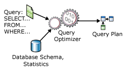
A SELECT statement is non-procedural; it doesn't state the exact steps that the database server should use to retrieve the requested data. This declarative behavior means that the database server must analyze the statement and the database to determine the most efficient way to extract the requested data. This process is referred to as query plan optimization. The component that performs this task is the Query Optimizer. The input to the Query Optimizer consists of the query, the database schema (object definitions), and the object statistics. The output of the Query Optimizer is a query execution plan, sometimes referred to as a query plan or execution plan. The contents of an execution plan are described in more detail in Execution plan caching and reuse.

The following diagram illustrates the inputs and outputs of the Query Optimizer during optimization of a single SELECT statement:

A SELECT statement defines only:

• The format of the result set. This is specified mostly in the select list. However, other clauses such as ORDER BY and GROUP BY also affect the final form of the result set.
• The tables that contain the source data. This is specified in the FROM clause.
• How the tables are logically related for the purposes of the SELECT statement. This is defined in the join expression, which might appear in the WHERE clause or in an ON clause following FROM.
• The conditions that the rows in the source tables must satisfy to qualify for the SELECT statement. These are specified in the WHERE and HAVING clauses.

A query execution plan defines:

• The sequence in which the source tables are accessed.

  Typically, the database server can access the base tables in many sequences to build the result set. For example, if the SELECT statement references three tables, the database server could first access TableA, use the data from TableA to extract matching rows from TableB, and then use the data from TableB to extract data from TableC. The other sequences in which the database server could access the tables are:

  TableC, TableB, TableA, or
  TableB, TableA, TableC, or
  TableB, TableC, TableA, or
  TableC, TableA, TableB

• The methods used to extract data from each table.

  Generally, there are different methods for accessing the data in each table. If only a few rows with specific key values are required, the database server can quickly look up rows or scan a small index range. If all the rows in the table are required, the database server can instead scan the entire table or index. If all the rows in a table are required but there's an index whose key columns are in an ORDER BY, performing an index scan instead of a table scan might save a separate sort of the result set. If a table is very small, full scans might be the most efficient method for almost all access to the table.

• The methods used to compute calculations, and how to filter, aggregate, and sort data from each table.

  As data is accessed from tables, different methods perform calculations over data such as computing scalar values, and aggregate and sort data as defined in the query text. For example, when using a GROUP BY or ORDER BY clause, and how to filter data, for example when using a WHERE or HAVING clause.

The process of selecting one execution plan from potentially many possible plans is referred to as optimization. The Query Optimizer is one of the most important components of the Database Engine. While the Query Optimizer uses some overhead to analyze the query and select a plan, this overhead is typically saved several-fold when the Query Optimizer picks an efficient execution plan. For example, two construction companies can be given identical blueprints for a house. If one company spends a few days at the beginning to plan how to build the house, and the other company begins building without planning, the company that takes the time to plan their project probably finishes first.

The Query Optimizer is a cost-based optimizer. Each possible execution plan has an associated cost in terms of the amount of computing resources used. The Query Optimizer must analyze the possible plans and choose the one with the lowest estimated cost. Some complex statements have thousands of possible execution plans. In these cases, the Query Optimizer doesn't analyze all possible combinations. Instead, it uses complex algorithms to find an execution plan that has a cost reasonably close to the minimum possible cost.

The Query Optimizer doesn't necessarily choose the execution plan with the lowest estimated cost. It finds a plan with a reasonable estimated cost within the time available for optimization. A parallel execution plan might use more resources than a serial plan while reducing the estimated elapsed time.

The SQL Server Query Optimizer relies on statistics when it estimates the resource costs of different methods for extracting information from a table or index. Statistics are kept for columns and indexes, and hold information on the density¹ of the underlying data. This information indicates the selectivity of the values in a particular index or column. For example, in a table representing cars, many cars have the same manufacturer, but each car has a unique vehicle identification number (VIN). An index on the VIN is more selective than an index on the manufacturer, because VIN has lower density than manufacturer. If the index statistics aren't current, the Query Optimizer might not make the best choice for the current state of the table. For more information about densities, see Statistics.

¹ Density defines the distribution of unique values that exist in the data, or the average number of duplicate values for a given column. As density decreases, selectivity of a value increases.

The Query Optimizer is important because it enables the database server to dynamically adjust to changing conditions in the database without requiring input from a developer or database administrator. This feature enables developers to focus on describing the final result of the query. They can trust the Query Optimizer to build an efficient execution plan for the state of the database every time the query plan for a statement is optimized.

Note

SQL Server Management Studio has three options to display execution plans:

• The Estimated Execution Plan, which is the compiled plan, as produced by the Query Optimizer.
• The Actual Execution Plan, which is the same as the compiled plan plus its execution context. This context includes runtime information available after the execution completes, such as execution warnings, or in newer versions of the Database Engine, the elapsed and CPU time used during execution.
• The Live Query Statistics, which is the same as the compiled plan plus its execution context. This context includes runtime information during execution progress, and is updated every second. Runtime information includes, for example, the actual number of rows flowing through the operators.

Process a SELECT statement

The Database Engine processes a single SELECT statement by following these steps:

1. The parser scans the SELECT statement and breaks it into logical units such as keywords, expressions, operators, and identifiers.
2. A query tree, sometimes referred to as a sequence tree, is built describing the logical steps needed to transform the source data into the format required by the result set.
3. The Query Optimizer analyzes different ways to access the source tables. It selects the series of steps that returns the results fastest while using fewer resources. It updates the query tree to record this exact series of steps. The final, optimized version of the query tree is called the execution plan.
4. The relational engine starts executing the plan. As it processes steps that need data from the base tables, it requests the required rowsets from the storage engine.
5. The relational engine processes the data returned from the storage engine into the format defined for the result set and returns the result set to the client.

Constant folding and expression evaluation

The Database Engine evaluates some constant expressions early to improve query performance. This optimization technique used by the Query Optimizer aims to simplify expressions at compile time rather than at runtime. It involves evaluating constant expressions during query compilation so that the resulting execution plan is more efficient. This process is referred to as constant folding. A constant is a T-SQL literal, such as 3, 'ABC', '2025-12-31', 1.0e3, or 0x12345678. For example, take this query:

SELECT *
FROM Orders
WHERE OrderDate < DATEADD(day, 30 * 12, '2025-01-01');

Here, 30 * 12 is a constant expression. The Database Engine evaluates this expression during compilation, and can rewrite the query internally as:

SELECT *
FROM Orders
WHERE OrderDate < DATEADD(day, 360, '2025-01-01');

Foldable expressions

The Database Engine uses constant folding with the following types of expressions:

• Arithmetic expressions, such as 1 + 1 and 5 / 3 * 2, that contain only constants.
• Logical expressions, such as 1 = 1 and 1 > 2 AND 3 > 4, that contain only constants.
• Built-in functions that the Database Engine considers foldable, including CAST and CONVERT. Generally, an intrinsic function is foldable if it's a function of its inputs only and not other contextual information, such as SET options, language settings, database options, and encryption keys. Nondeterministic functions aren't foldable. Deterministic built-in functions are foldable, with some exceptions.
• Deterministic methods of CLR user-defined types and deterministic scalar-valued CLR user-defined functions. For more information, see Constant Folding for CLR User-Defined Functions and Methods.

Note

An exception is made for large object types. If the output type of the folding process is a large object type (text, ntext, image, nvarchar(max), varchar(max), varbinary(max), json, or xml), the Database Engine doesn't fold the expression.

Nonfoldable expressions

All other expression types aren't foldable. In particular, the following types of expressions aren't foldable:

• Nonconstant expressions such as an expression whose result depends on the value of a column.
• Expressions whose results depend on a local variable or parameter, such as @x.
• Nondeterministic functions.
• User-defined T-SQL functions.
• Expressions whose results depend on language settings.
• Expressions whose results depend on SET options.
• Expressions whose results depend on server configuration options.

Examples of foldable and nonfoldable constant expressions

Consider the following query:

USE AdventureWorks2025;
GO

SELECT *
FROM Sales.SalesOrderHeader AS s
     INNER JOIN Sales.SalesOrderDetail AS d
         ON s.SalesOrderID = d.SalesOrderID
WHERE TotalDue > 117.00 + 1000.00;

If the PARAMETERIZATION database option isn't set to FORCED for this query, the expression 117.00 + 1000.00 is evaluated and replaced by its result, 1117.00, before the query is compiled. Benefits of this constant folding include:

• The expression doesn't have to be evaluated repeatedly at run time.
• The value of the expression after it's evaluated is used by the Query Optimizer to estimate the size of the result set of the portion of the query TotalDue > 117.00 + 1000.00.

On the other hand, if dbo.f is a user-defined scalar function, the expression dbo.f(100) isn't folded, because the Database Engine doesn't fold expressions that involve user-defined functions, even if they're deterministic. For more information about parameterization, see Forced parameterization.

Expression evaluation

In addition, some expressions that aren't constant folded but whose arguments are known at compile time, whether the arguments are parameters or constants, are evaluated by the result-set size (cardinality) estimator that is part of the optimizer during optimization.

Specifically, the following built-in functions and special operators are evaluated at compile time if all their inputs are known: UPPER, LOWER, RTRIM, DATEPART( YY only ), GETDATE, CAST, and CONVERT. The following operators are also evaluated at compile time if all their inputs are known:

• Arithmetic operators: +, -, *, /, unary -
• Logical operators: AND, OR, NOT
• Comparison operators: <, >, <=, >=, <>, LIKE, IS NULL, IS NOT NULL

No other functions or operators are evaluated by the Query Optimizer during cardinality estimation.

Examples of compile-time expression evaluation

Consider this stored procedure:

USE AdventureWorks2025;
GO

CREATE PROCEDURE MyProc
(
    @d DATETIME
)
AS
SELECT COUNT(*)
FROM Sales.SalesOrderHeader
WHERE OrderDate > @d + 1;

During optimization of the SELECT statement in the procedure, the Query Optimizer tries to evaluate the expected cardinality of the result set for the condition OrderDate > @d + 1. The expression @d + 1 isn't constant-folded, because @d is a parameter. However, at optimization time, the value of the parameter is known. This value allows the Query Optimizer to accurately estimate the size of the result set, which helps it select a good query plan.

Now consider an example similar to the previous one, except that a local variable @d2 replaces @d + 1 in the query and the expression is evaluated in a SET statement instead of in the query.

USE AdventureWorks2025;
GO

CREATE PROCEDURE MyProc2
(
    @d DATETIME
)
AS
BEGIN
    DECLARE @d2 AS DATETIME;
    SET @d2 = @d + 1;
    SELECT COUNT(*)
    FROM Sales.SalesOrderHeader
    WHERE OrderDate > @d2;
END

When the SELECT statement in MyProc2 is optimized in the Database Engine, the value of @d2 isn't known. Therefore, the Query Optimizer uses a default estimate for the selectivity of OrderDate > @d2 (in this case 30 percent).

Process other statements

The basic steps for processing a SELECT statement apply to other T-SQL statements such as INSERT, UPDATE, and DELETE. Both UPDATE and DELETE statements must target the set of rows to modify or delete. The process of identifying these rows is the same process used to identify the source rows that contribute to the result set of a SELECT statement. Both UPDATE and INSERT statements might contain embedded SELECT statements that provide the data values to update or insert.

Even Data Definition Language (DDL) statements, such as CREATE PROCEDURE or ALTER TABLE, resolve to a series of relational operations on the system catalog tables and sometimes (such as ALTER TABLE ADD COLUMN) against the data tables.

Worktables

The relational engine might need to build a worktable to perform a logical operation specified in a T-SQL statement. Worktables are internal tables that hold intermediate results. Worktables are generated for certain GROUP BY, ORDER BY, or UNION queries. For example, if an ORDER BY clause references columns that aren't covered by any indexes, the relational engine might need to generate a worktable to sort the result set into the order requested. Worktables are also sometimes used as spools that temporarily hold the result of executing a part of a query plan. Worktables are built in tempdb, and then dropped automatically when they're no longer needed.

View resolution

The Database Engine query processor treats indexed and nonindexed views differently:

• The database stores the rows of an indexed view in the same format as a table. If the Query Optimizer decides to use an indexed view in a query plan, it treats the indexed view the same way as a base table.
• Only the definition of a nonindexed view is stored, not the rows of the view. The Query Optimizer incorporates the logic from the view definition into the execution plan it builds for the T-SQL statement that references the nonindexed view.

The logic the Query Optimizer uses to decide when to use an indexed view is similar to the logic it uses to decide when to use an index on a table. If the data in the indexed view covers all or part of the T-SQL statement, and the Query Optimizer determines that an index on the view is the low-cost access path, it chooses the index regardless of whether the query references the view by name.

When a T-SQL statement references a nonindexed view, the parser and Query Optimizer analyze the source of both the T-SQL statement and the view and then resolve them into a single execution plan. The T-SQL statement and the view don't have separate plans.

For example, consider the following view:

USE AdventureWorks2025;
GO

CREATE VIEW EmployeeName AS
    SELECT h.BusinessEntityID,
           p.LastName,
           p.FirstName
    FROM HumanResources.Employee AS h
         INNER JOIN Person.Person AS p
             ON h.BusinessEntityID = p.BusinessEntityID;
GO

Based on this view, both of these T-SQL statements perform the same operations on the base tables and produce the same results:

USE AdventureWorks2025;
GO

/* SELECT referencing the EmployeeName view. */
SELECT LastName AS EmployeeLastName,
       SalesOrderID,
       OrderDate
FROM Sales.SalesOrderHeader AS soh
     INNER JOIN dbo.EmployeeName AS EmpN
         ON (soh.SalesPersonID = EmpN.BusinessEntityID)
WHERE OrderDate > '20230531';

/* SELECT referencing the Person and Employee tables directly. */
SELECT LastName AS EmployeeLastName,
       SalesOrderID,
       OrderDate
FROM HumanResources.Employee AS e
     INNER JOIN Sales.SalesOrderHeader AS soh
         ON soh.SalesPersonID = e.BusinessEntityID
     INNER JOIN Person.Person AS p
         ON e.BusinessEntityID = p.BusinessEntityID
WHERE OrderDate > '20230531';

The SQL Server Management Studio (SSMS) Showplan feature shows that the relational engine builds the same execution plan for both of these SELECT statements.

Use hints with views

If you place hints on views in a query, they might conflict with other hints that are discovered when the view expands to access its base tables. When this conflict occurs, the query returns an error. For example, consider the following view that contains a table hint in its definition:

USE AdventureWorks2025;
GO

CREATE VIEW Person.AddrState
WITH SCHEMABINDING AS
    SELECT a.AddressID,
           a.AddressLine1,
           s.StateProvinceCode,
           s.CountryRegionCode
    FROM Person.Address AS a WITH (NOLOCK), Person.StateProvince AS s
    WHERE a.StateProvinceID = s.StateProvinceID;

Now suppose you enter this query:

SELECT AddressID,
       AddressLine1,
       StateProvinceCode,
       CountryRegionCode
FROM Person.AddrState WITH (SERIALIZABLE)
WHERE StateProvinceCode = 'WA';

The query fails, because the SERIALIZABLE hint on the Person.AddrState view propagates to both the Person.Address and Person.StateProvince tables in the view when it's expanded. However, expanding the view also reveals the NOLOCK hint on Person.Address. Because the SERIALIZABLE and NOLOCK hints conflict, the resulting query is incorrect.

The PAGLOCK, NOLOCK, ROWLOCK, TABLOCK, and TABLOCKX table hints conflict with each other, as do the HOLDLOCK, NOLOCK, READCOMMITTED, REPEATABLEREAD, and SERIALIZABLE table hints.

Hints can propagate through levels of nested views. For example, suppose a query applies the HOLDLOCK hint on a view v1. When v1 is expanded, you find that view v2 is part of its definition. v2's definition includes a NOLOCK hint on one of its base tables. But this table also inherits the HOLDLOCK hint from the query on view v1. Because the NOLOCK and HOLDLOCK hints conflict, the query fails.

When you use the FORCE ORDER hint in a query that contains a view, the position of the view in the ordered construct determines the join order of the tables within the view. For example, the following query selects from three tables and a view:

SELECT * FROM Table1, Table2, View1, Table3
WHERE Table1.Col1 = Table2.Col1
    AND Table2.Col1 = View1.Col1
    AND View1.Col2 = Table3.Col2;
OPTION (FORCE ORDER);

And View1 is defined as shown in the following example:

CREATE VIEW View1 AS
    SELECT Colx,
           Coly
    FROM TableA, TableB
    WHERE TableA.ColZ = TableB.Colz;

The join order in the query plan is Table1, Table2, TableA, TableB, Table3.

Resolve indexes on views

As with any index, the Database Engine chooses to use an indexed view in its query plan only if the Query Optimizer determines it's beneficial to do so.

You can create indexed views in any edition of the Database Engine. In some editions, the Query Optimizer automatically considers the indexed view, while in other editions you need to use the NOEXPAND table hint. Automatic use of an indexed view by the Query Optimizer is supported only in specific editions of SQL Server.

Note

Azure SQL Database and Azure SQL Managed Instance support automatic use of indexed views without specifying the NOEXPAND hint.

The Query Optimizer uses an indexed view when the following conditions are met:

• These session options are set to ON:
  • ANSI_NULLS
  • ANSI_PADDING
  • ANSI_WARNINGS
  • ARITHABORT
  • CONCAT_NULL_YIELDS_NULL
  • QUOTED_IDENTIFIER
• The NUMERIC_ROUNDABORT session option is set to OFF.
• The Query Optimizer finds a match between the view index columns and elements in the query, such as:
  • Search condition predicates in the WHERE clause
  • Join operations
  • Aggregate functions
  • GROUP BY clauses
  • Table references
• The estimated cost for using the index has the lowest cost of any access mechanisms considered by the Query Optimizer.
• Every table referenced in the query (either directly, or by expanding a view to access its underlying tables) that corresponds to a table reference in the indexed view must have the same set of hints applied on it in the query.

Note

The READCOMMITTED and READCOMMITTEDLOCK hints are always considered different hints in this context, regardless of the current transaction isolation level.

Other than the requirements for the SET options and table hints, these are the same rules that the Query Optimizer uses to determine whether a table index covers a query. You don't need to specify anything else in the query for an indexed view to be used.

A query doesn't have to explicitly reference an indexed view in the FROM clause for the Query Optimizer to use the indexed view. If the query contains references to columns in the base tables that are also present in the indexed view, and the Query Optimizer estimates that using the indexed view provides the lowest cost access mechanism, the Query Optimizer chooses the indexed view, similar to the way it chooses base table indexes when they aren't directly referenced in a query. The Query Optimizer can choose the view when it contains columns that aren't referenced by the query, as long as the view offers the lowest cost option for covering one or more of the columns specified in the query.

The Query Optimizer treats an indexed view referenced in the FROM clause as a standard view. The Query Optimizer expands the definition of the view into the query at the start of the optimization process. Then, indexed view matching is performed. The indexed view can be used in the final execution plan selected by the Query Optimizer, or instead, the plan might materialize necessary data from the view by accessing the base tables referenced by the view. The Query Optimizer chooses the lowest-cost alternative.

Use hints with indexed views

You can prevent view indexes from being used for a query by using the EXPAND VIEWS query hint, or you can use the NOEXPAND table hint to force the use of an index for an indexed view specified in the FROM clause of a query. However, you should let the Query Optimizer dynamically determine the best access methods to use for each query. Limit your use of EXPAND and NOEXPAND to specific cases where testing has shown that they improve performance significantly.

• The EXPAND VIEWS option specifies that the Query Optimizer not use any view indexes for the whole query.

• When you specify NOEXPAND for a view, the Query Optimizer considers using any indexes defined on the view. NOEXPAND specified with the optional INDEX() clause forces the Query Optimizer to use the specified indexes. You can specify NOEXPAND only for an indexed view and can't specify it for a view that isn't indexed. Automatic use of an indexed view by the Query Optimizer is supported only in specific editions of SQL Server.

  Note

  Azure SQL Database and Azure SQL Managed Instance support automatic use of indexed views without specifying the NOEXPAND hint.

When neither NOEXPAND nor EXPAND VIEWS is specified in a query that contains a view, the view is expanded to access underlying tables. If the query that makes up the view contains any table hints, these hints are propagated to the underlying tables. (This process is explained in more detail in View resolution.) As long as the set of hints that exists on the underlying tables of the view are identical to each other, the query is eligible to be matched with an indexed view. Most of the time, these hints match each other, because they're inherited directly from the view. However, if the query references tables instead of views, and the hints applied directly on these tables aren't identical, then such a query isn't eligible for matching with an indexed view. If the INDEX, PAGLOCK, ROWLOCK, TABLOCKX, UPDLOCK, or XLOCK hints apply to the tables referenced in the query after view expansion, the query isn't eligible for indexed view matching.

If a table hint in the form of INDEX ( index_val [ ,...n] ) references a view in a query and you don't also specify the NOEXPAND hint, the index hint is ignored. To specify use of a particular index, use NOEXPAND.

Generally, when the Query Optimizer matches an indexed view to a query, it applies any hints specified on the tables or views in the query directly to the indexed view. If the Query Optimizer chooses not to use an indexed view, it propagates any hints directly to the tables referenced in the view. For more information, see View resolution. This propagation doesn't apply to join hints. They are applied only in their original position in the query. The Query Optimizer doesn't consider join hints when matching queries to indexed views. If a query plan uses an indexed view that matches part of a query that contains a join hint, the join hint isn't used in the plan.

Hints aren't allowed in the definitions of indexed views. The Database Engine ignores hints inside indexed view definitions when maintaining them, or when executing queries that use indexed views.

For more information, see Table Hints.

Resolve distributed partitioned views

The Database Engine query processor optimizes the performance of distributed partitioned views. The most important aspect of distributed partitioned view performance is minimizing the amount of data transferred between member servers.

The Database Engine builds intelligent, dynamic plans that make efficient use of distributed queries to access data from remote member tables:

• The Query Processor first uses OLE DB to retrieve the check constraint definitions from each member table. This method allows the query processor to map the distribution of key values across the member tables.
• The Query Processor compares the key ranges specified in a T-SQL statement WHERE clause to the map that shows how the rows are distributed in the member tables. The query processor then builds a query execution plan that uses distributed queries to retrieve only those remote rows that are required to complete the T-SQL statement. The execution plan is also built in such a way that any access to remote member tables, for either data or metadata, is delayed until the information is required.

For example, consider a system where a Customers table is partitioned across Server1 (CustomerID from 1 through 3299999), Server2 (CustomerID from 3300000 through 6599999), and Server3 (CustomerID from 6600000 through 9999999).

Consider the execution plan built for this query executed on Server1:

SELECT *
FROM CompanyData.dbo.Customers
WHERE CustomerID BETWEEN 3200000 AND 3400000;

The execution plan for this query extracts the rows with CustomerID key values from 3200000 through 3299999 from the local member table, and issues a distributed query to retrieve the rows with key values from 3300000 through 3400000 from Server2.

The Database Engine Query Processor can also build dynamic logic into query execution plans for T-SQL statements in which the key values aren't known when the plan must be built. For example, consider this stored procedure:

CREATE PROCEDURE GetCustomer
(
    @CustomerIDParameter INT
)
AS
SELECT *
FROM CompanyData.dbo.Customers
WHERE CustomerID = @CustomerIDParameter;

The Database Engine can't predict what key value is supplied by the @CustomerIDParameter parameter every time the procedure executes. Because the key value can't be predicted, the query processor also can't predict which member table it has to access. To handle this case, the Database Engine builds an execution plan that has conditional logic, referred to as dynamic filters, to control which member table is accessed, based on the input parameter value. Assuming the GetCustomer stored procedure was executed on Server1, the execution plan logic can be represented as shown in the following output:

IF @CustomerIDParameter BETWEEN 1 and 3299999
   Retrieve row from local table CustomerData.dbo.Customer_33
ELSE IF @CustomerIDParameter BETWEEN 3300000 and 6599999
   Retrieve row from linked table Server2.CustomerData.dbo.Customer_66
ELSE IF @CustomerIDParameter BETWEEN 6600000 and 9999999
   Retrieve row from linked table Server3.CustomerData.dbo.Customer_99

The Database Engine sometimes builds these types of dynamic execution plans even for queries that aren't parameterized. The Query Optimizer can parameterize a query so that the execution plan can be reused. If the Query Optimizer parameterizes a query referencing a partitioned view, the Query Optimizer can no longer assume the required rows come from a specified base table. It then has to use dynamic filters in the execution plan.

Stored procedure and trigger execution

The Database Engine stores only the source for stored procedures and triggers. When a stored procedure or trigger is first executed, the source is compiled into an execution plan. If the stored procedure or trigger is again executed before the execution plan is aged from memory, the relational engine detects the existing plan and reuses it. If the plan ages out of memory, a new plan is built. This process is similar to the process the Database Engine follows for all T-SQL statements. The main performance advantage that stored procedures and triggers have in the Database Engine compared with batches of dynamic T-SQL is that their T-SQL statements are always the same. Therefore, the relational engine easily matches them with any existing execution plans. Stored procedure and trigger plans are easily reused.

The execution plan for stored procedures and triggers is executed separately from the execution plan for the batch calling the stored procedure or firing the trigger. This separation allows for greater reuse of the stored procedure and trigger execution plans.

Execution plan caching and reuse

The Database Engine uses memory to store both execution plans and data buffers. The percentage of memory allocated to execution plans or data buffers is adjusted dynamically, depending on the state of the system. The portion of memory that stores execution plans is called the plan cache.

Plan cache stores

The plan cache has two stores for all compiled plans:

• The Object Plans cache store (OBJCP), for plans related to persisted objects, such as stored procedures, functions, and triggers.
• The SQL Plans cache store (SQLCP), for plans related to autoparameterized, dynamic, or prepared queries.

The following query provides information about memory usage for these two cache stores:

SELECT *
FROM sys.dm_os_memory_clerks
WHERE name LIKE '%plans%';

The plan cache has two additional stores that don't store plans:

• The Bound Trees cache store (PHDR), for data structures used during plan compilation for views, constraints, and defaults. These structures are known as bound trees or algebrizer trees.
• The Extended Stored Procedures cache store (XPROC), for predefined system procedures, like sp_executesql or xp_cmdshell. These stored procedures use a DLL instead of T-SQL statements. The cached structure contains only the function name and the DLL name where the procedure is implemented.

Execution plan components

Database Engine execution plans have the following main components:

Compiled plan (or query plan)

The query plan produced by the compilation process is mostly a re-entrant, read-only data structure used by any number of users. It stores information about:

• Physical operators that implement the operation described by logical operators.

• The order of these operators, which determines the order in which data is accessed, filtered, and aggregated.

• The number of estimated rows flowing through the operators.

  Note

  The query plan also stores information about the statistics objects used for Cardinality Estimation.

• What support objects must be created, such as worktables or workfiles in tempdb.

The query plan doesn't store any user context or runtime information. The Database Engine determines the number of worker threads each time it retrieves a plan from the plan cache. A cached parallel plan can also run serially.

Execution context

Each user that currently executes the query has a data structure that holds the data specific to their execution, such as parameter values. This data structure is called the execution context. The execution context data structures are reused, but their content isn't. If another user executes the same query, the data structures are reinitialized with the context for the new user.

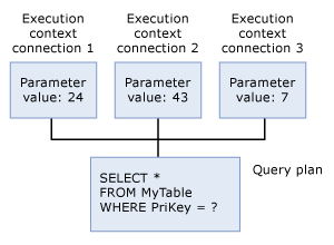
Reuse plans for identical statements

When the Database Engine executes any T-SQL statement, it first looks through the plan cache to verify that an existing execution plan for the same T-SQL statement exists. The T-SQL statement qualifies as existing if it literally matches a previously executed T-SQL statement with a cached plan, character by character. The Database Engine reuses any existing plan it finds, saving the overhead of recompiling the T-SQL statement. If no execution plan exists, the Database Engine generates a new execution plan for the query.

Note

The plan cache doesn't persist execution plans for some T-SQL statements, such as bulk operation statements running on rowstore or statements containing large string literals. These plans exist only while the query is running.

The Database Engine uses an efficient algorithm to find any existing execution plans for any specific T-SQL statement. In most systems, the minimal resources that this scan uses are less than the resources that are saved by reusing existing plans instead of compiling every T-SQL statement.

The algorithms to match new T-SQL statements to existing, unused execution plans in the plan cache require that all object references be fully qualified. For example, assume that Person is the default schema for the user executing the following SELECT statements. While this example doesn't require that you fully qualify the Person table to execute, it means that the second statement doesn't match an existing plan, but the third statement does match:

USE AdventureWorks2025;
GO

SELECT *
FROM Person;
GO

SELECT *
FROM Person.Person;
GO

SELECT *
FROM Person.Person;
GO

Changing any of the following SET options for a given execution affects the ability to reuse plans, because the Database Engine performs constant folding and these options affect the results of such expressions:

• ANSI_DEFAULTS
• ANSI_NULL_DFLT_OFF
• ANSI_NULL_DFLT_ON
• ANSI_NULLS
• ANSI_PADDING
• ANSI_WARNINGS
• ARITHABORT
• CONCAT_NULL_YIELDS_NULL
• DATEFIRST
• DATEFORMAT
• FORCEPLAN
• LANGUAGE
• NO_BROWSETABLE
• NUMERIC_ROUNDABORT
• QUOTED_IDENTIFIER

Cache multiple plans for the same query

Queries and execution plans are uniquely identifiable in the Database Engine, much like a fingerprint:

• The query plan hash is a binary hash value calculated on the execution plan for a given query, and used to uniquely identify similar execution plans.
• The query hash is a binary hash value calculated on the T-SQL text of a query, and is used to uniquely identify queries.

You can retrieve a compiled plan from the plan cache by using a plan handle. This transient identifier stays constant only while the plan stays in the cache. The plan handle is a hash value derived from the compiled plan of the entire batch. The plan handle for a compiled plan stays the same even if one or more statements in the batch get recompiled.

Note

If you compile a plan for a batch instead of a single statement, you can use the plan handle and statement offsets to get the plan for individual statements in the batch. The sys.dm_exec_requests DMV contains the statement_start_offset and statement_end_offset columns for each record. These columns refer to the currently executing statement of a currently executing batch or persisted object. For more information, see sys.dm_exec_requests. The sys.dm_exec_query_stats DMV also contains these columns for each record. These columns refer to the position of a statement within a batch or persisted object. For more information, see sys.dm_exec_query_stats.

The actual T-SQL text of a batch is stored in a separate memory space from the plan cache, called the SQL Manager cache (SQLMGR). You can retrieve the T-SQL text for a compiled plan from the SQL Manager cache by using a SQL handle. This transient identifier remains constant only while at least one plan that references it remains in the plan cache. The SQL handle is a hash value derived from the entire batch text, and is guaranteed to be unique for every batch.

Note

Like a compiled plan, the T-SQL text is stored per batch, including the comments. The SQL handle contains the MD5 hash of the entire batch text and is guaranteed to be unique for every batch.

The following query provides information about memory usage for the SQL Manager cache:

SELECT *
FROM sys.dm_os_memory_objects
WHERE type = 'MEMOBJ_SQLMGR';

There's a one-to-many relationship between a SQL handle and plan handles. This condition occurs when the cache key for the compiled plans is different. This difference might occur due to change in SET options between two executions of the same batch.

Consider the following stored procedure:

USE WideWorldImporters;
GO

CREATE PROCEDURE usp_SalesByCustomer
(
    @CID INT
)
AS
SELECT *
FROM Sales.Customers
WHERE CustomerID = @CID;
GO

SET ANSI_DEFAULTS ON;
GO

EXECUTE usp_SalesByCustomer 10;
GO

Verify what you can find in the plan cache by using the following query:

SELECT cp.memory_object_address,
       cp.objtype,
       refcounts,
       usecounts,
       qs.query_plan_hash,
       qs.query_hash,
       qs.plan_handle,
       qs.sql_handle
FROM sys.dm_exec_cached_plans AS cp
CROSS APPLY sys.dm_exec_sql_text(cp.plan_handle)
CROSS APPLY sys.dm_exec_query_plan(cp.plan_handle)
     INNER JOIN sys.dm_exec_query_stats AS qs
         ON qs.plan_handle = cp.plan_handle
WHERE text LIKE '%usp_SalesByCustomer%';
GO

Here's the result set.

memory_object_address    objtype   refcounts   usecounts   query_plan_hash    query_hash
---------------------   -------  ---------  ---------  ------------------ ------------------
0x000001CC6C534060        Proc      2           1           0x3B4303441A1D7E6D 0xA05D5197DA1EAC2D

plan_handle
------------------------------------------------------------------------------------------
0x0500130095555D02D022F111CD01000001000000000000000000000000000000000000000000000000000000

sql_handle
------------------------------------------------------------------------------------------
0x0300130095555D02C864C10061AB000001000000000000000000000000000000000000000000000000000000

Now execute the stored procedure with a different parameter, with no other changes to execution context:

EXECUTE usp_SalesByCustomer 8;
GO

Verify again what you can find in the plan cache. Here's the result set.

memory_object_address    objtype   refcounts   usecounts   query_plan_hash    query_hash
---------------------   -------  ---------  ---------  ------------------ ------------------
0x000001CC6C534060        Proc      2           2           0x3B4303441A1D7E6D 0xA05D5197DA1EAC2D

plan_handle
------------------------------------------------------------------------------------------
0x0500130095555D02D022F111CD01000001000000000000000000000000000000000000000000000000000000

sql_handle
------------------------------------------------------------------------------------------
0x0300130095555D02C864C10061AB000001000000000000000000000000000000000000000000000000000000

Notice the usecounts value increases to 2, which means the same cached plan is reused as-is, because the execution context data structures are reused. Now change the SET ANSI_DEFAULTS option and execute the stored procedure by using the same parameter.

SET ANSI_DEFAULTS OFF;
GO

EXECUTE usp_SalesByCustomer 8;
GO

Verify again what you can find in the plan cache. Here's the result set.

memory_object_address    objtype   refcounts   usecounts   query_plan_hash    query_hash
---------------------   -------  ---------  ---------  ------------------ ------------------
0x000001CD01DEC060        Proc      2           1           0x3B4303441A1D7E6D 0xA05D5197DA1EAC2D
0x000001CC6C534060        Proc      2           2           0x3B4303441A1D7E6D 0xA05D5197DA1EAC2D

plan_handle
------------------------------------------------------------------------------------------
0x0500130095555D02B031F111CD01000001000000000000000000000000000000000000000000000000000000
0x0500130095555D02D022F111CD01000001000000000000000000000000000000000000000000000000000000

sql_handle
------------------------------------------------------------------------------------------
0x0300130095555D02C864C10061AB000001000000000000000000000000000000000000000000000000000000
0x0300130095555D02C864C10061AB000001000000000000000000000000000000000000000000000000000000

Notice there are now two entries in the sys.dm_exec_cached_plans DMV output:

• The usecounts column shows the value 1 in the first record. This value represents the plan executed once with SET ANSI_DEFAULTS OFF.
• The usecounts column shows the value 2 in the second record. This value represents the plan executed with SET ANSI_DEFAULTS ON, because it was executed twice.
• The different memory_object_address refers to a different execution plan entry in the plan cache. However, the sql_handle value is the same for both entries because they refer to the same batch.
  • The execution with ANSI_DEFAULTS set to OFF has a new plan_handle, and it's available for reuse for calls that have the same set of SET options. The new plan handle is necessary because the execution context was reinitialized due to changed SET options. But that change doesn't trigger a recompile: both entries refer to the same plan and query, as evidenced by the same query_plan_hash and query_hash values.

This situation means that you have two plan entries in the cache corresponding to the same batch. It underscores the importance of making sure that the plan cache affecting SET options are the same when the same queries are executed repeatedly. This approach optimizes plan reuse and keeps the plan cache size to its required minimum.

Tip

A common pitfall is that different clients can have different default values for the SET options. For example, a connection made through SQL Server Management Studio automatically sets QUOTED_IDENTIFIER to ON, while SQLCMD sets QUOTED_IDENTIFIER to OFF. Executing the same queries from these two clients results in multiple plans (as described in the previous example).

Remove execution plans from the plan cache

Execution plans stay in the plan cache as long as there's enough memory to store them. When memory pressure exists, the SQL Server Database Engine uses a cost-based approach to decide which execution plans to remove from the plan cache. To make a cost-based decision, the SQL Server Database Engine increases and decreases a current cost variable for each execution plan based on the following factors.

When a user process inserts an execution plan into the cache, the user process sets the current cost equal to the original query compile cost. For ad hoc execution plans, the user process sets the current cost to zero. After that, each time a user process references an execution plan, it resets the current cost to the original compile cost. For ad hoc execution plans, the user process increases the current cost. For all plans, the maximum value for the current cost is the original compile cost.

When memory pressure exists, the SQL Server Database Engine removes execution plans from the plan cache. To determine which plans to remove, the SQL Server Database Engine repeatedly examines the state of each execution plan and removes plans when their current cost is zero. An execution plan with zero current cost isn't removed automatically when memory pressure exists. It's only removed when the SQL Server Database Engine examines the plan and the current cost is zero. When examining an execution plan, the SQL Server Database Engine pushes the current cost toward zero by decreasing the current cost if a query isn't currently using the plan.

The SQL Server Database Engine keeps examining the execution plans until it removes enough plans to satisfy memory requirements. While memory pressure exists, an execution plan might have its cost increased and decreased more than once. When memory pressure no longer exists, the SQL Server Database Engine stops decreasing the current cost of unused execution plans. All execution plans stay in the plan cache, even if their cost is zero.

The SQL Server Database Engine uses the resource monitor and user worker threads to free memory from the plan cache in response to memory pressure. The resource monitor and user worker threads can concurrently examine plans to decrease the current cost for each unused execution plan. The resource monitor removes execution plans from the plan cache when global memory pressure exists. It frees memory to enforce policies for system memory, process memory, resource pool memory, and maximum size for all caches.

The maximum size for all caches is a function of the buffer pool size and can't exceed the maximum server memory. For more information about configuring the maximum server memory, see the max server memory setting in sp_configure.

The user worker threads remove execution plans from the plan cache when single cache memory pressure exists. They enforce policies for maximum single cache size and maximum single cache entries.

The following examples illustrate which execution plans get removed from the plan cache:

• An execution plan is frequently referenced so that its cost never goes to zero. The plan stays in the plan cache and isn't removed unless there's memory pressure and the current cost is zero.
• An ad hoc execution plan is inserted and isn't referenced again before memory pressure exists. Since ad hoc plans are initialized with a current cost of zero, when the SQL Server Database Engine examines the execution plan, it sees the zero current cost and removes the plan from the plan cache. The ad hoc execution plan stays in the plan cache with a zero current cost when memory pressure doesn't exist.

To manually remove a single plan or all plans from the cache, use DBCC FREEPROCCACHE. You can also use DBCC FREESYSTEMCACHE to clear any cache, including plan cache. SQL Server 2016 (13.x) and later versions, use ALTER DATABASE SCOPED CONFIGURATION CLEAR PROCEDURE_CACHE to clear the procedure (plan) cache for the database in scope.

A change in some configuration settings through sp_configure and reconfigure also causes the removal of plans from the plan cache. You can find the list of these configuration settings in the Remarks section of the DBCC FREEPROCCACHE article. When you make this configuration change, the following informational message is written to the error log:

SQL Server has encountered %d occurrence(s) of cachestore flush for the '%s' cachestore (part of plan cache) due to some database maintenance or reconfigure operations.

Recompile execution plans

Certain changes in a database can make an execution plan inefficient or invalid. The Database Engine detects these changes and marks the plan as not valid. A new plan must then be recompiled for the next connection that executes the query. Conditions that invalidate a plan include:

• Changes to a table or view referenced by the query (ALTER TABLE and ALTER VIEW).
• Changes to a single procedure, which would drop all plans for that procedure from the cache (ALTER PROCEDURE).
• Changes to any indexes used by the execution plan.
• Updates to statistics used by the execution plan, whether explicitly generated by a statement such as UPDATE STATISTICS or generated automatically.
• Dropping an index used by the execution plan.
• An explicit call to sp_recompile.
• Large numbers of changes to keys (generated by INSERT or DELETE statements from other users that modify a table referenced by the query).
• For tables with triggers, if the number of rows in the inserted or deleted tables grows significantly.
• Executing a stored procedure by using the WITH RECOMPILE option.

Most recompilations are required either for statement correctness or to get potentially faster query execution plans.

When a statement within a batch triggers recompilation, only that statement is recompiled, not the entire batch. This rule applies whether the batch is submitted through a stored procedure, trigger, ad hoc batch, or prepared statement.

Statement-level recompilation benefits performance because, in most cases, a small number of statements cause recompilations and their associated penalties, in terms of CPU time and locks. These penalties are therefore avoided for the other statements in the batch that don't need recompilation.

The sql_statement_recompile extended event (XEvent) reports statement-level recompilations. This XEvent occurs when a statement-level recompilation is required by any kind of batch. This requirement includes stored procedures, triggers, ad hoc batches, and queries. Batches can be submitted through several interfaces, including sp_executesql, dynamic SQL, Prepare methods, or Execute methods.

The recompile_cause column of sql_statement_recompile XEvent contains an integer code that indicates the reason for the recompilation. The following list contains the possible reasons:

• Cursor options changed
• Deferred compile
• FOR BROWSE permission changed
• OPTION (RECOMPILE) requested
• Parameterized plan flushed
• Partitioned view changed
• Plan affecting database version changed
• Query notification environment changed
• Query Store missing the plan
• Query Store plan forcing failed
• Query Store plan forcing policy changed
• Remote rowset changed
• Schema changed
• SET option changed
• Statistics changed
• Temporary table changed

Note

When you set the AUTO_UPDATE_STATISTICS database option to ON, queries are recompiled when they target tables or indexed views whose statistics are updated or whose cardinalities change significantly since the last execution. This behavior applies to standard user-defined tables, temporary tables, and the inserted and deleted tables created by DML triggers.

Setting AUTO_UPDATE_STATISTICS to OFF stops these recompilations, but out-of-date statistics usually degrade query performance more than the recompilations do. For more information, see the AUTO_UPDATE_STATISTICS option. The inserted and deleted tables of DML INSTEAD OF triggers are created in tempdb, so they follow the AUTO_UPDATE_STATISTICS setting of tempdb.

Use explicit parameters for plan reuse

Using parameters, including named parameters in ADO.NET applications and parameter markers in OLE DB and ODBC applications, can increase the reuse of execution plans.

Warning

Always validate user input by testing type, length, format, and range. For more information, see SQL injection.

The only difference between the following two SELECT statements is the values that are compared in the WHERE clause:

SELECT *
FROM Production.Product
WHERE ProductSubcategoryID = 1;

SELECT *
FROM Production.Product
WHERE ProductSubcategoryID = 4;

The only difference between the execution plans for these queries is the value stored for the comparison against the ProductSubcategoryID column. While the goal is for the Database Engine to always recognize that the statements generate essentially the same plan and reuse the plans, the Database Engine sometimes doesn't detect this similarity in complex T-SQL statements.

Separating constants from the T-SQL statement by using parameters helps the relational engine recognize duplicate plans. Use parameters in the following ways:

• In T-SQL, use sp_executesql:

  DECLARE @MyIntParm AS INT;
  
  SET @MyIntParm = 1;
  
  EXECUTE sp_executesql N'SELECT *
     FROM AdventureWorks2025.Production.Product
     WHERE ProductSubcategoryID = @Parm', N'@Parm INT', @MyIntParm;
  

  This method is recommended for T-SQL scripts, stored procedures, or triggers that generate SQL statements dynamically.

• ADO.NET with SqlClient uses named parameters, such as @Parm. OLE DB and ODBC use parameter markers. Parameter markers are question marks (?) that replace a constant in a SQL statement and are bound to a program variable. For example, you would do the following in an ODBC application:

  • Use SQLBindParameter to bind an integer variable to the first parameter marker in a SQL statement.

  • Put the integer value in the variable.

  • Execute the statement, specifying the parameter marker (?):

    SQLExecDirect(hstmt,
      "SELECT *
      FROM AdventureWorks2025.Production.Product
      WHERE ProductSubcategoryID = ?",
      SQL_NTS);
    

  The SQL Server Native Client OLE DB Provider and the SQL Server Native Client ODBC driver use sp_executesql to send statements to SQL Server when parameter markers are used in applications.

• Write stored procedures, which use parameters by design.

If you don't explicitly build parameters into the design of your applications, you can also rely on the Query Optimizer to automatically parameterize certain queries by using the default behavior of simple parameterization. Alternatively, you can force the Query Optimizer to consider parameterizing all queries in the database by setting the PARAMETERIZATION option of the ALTER DATABASE statement to FORCED.

Simple parameterization

In the Database Engine, using parameters or parameter markers in T-SQL statements increases the ability of the relational engine to match new T-SQL statements with existing, previously compiled execution plans.

Warning

Always validate user input by testing type, length, format, and range. For more information, see SQL injection.

If a T-SQL statement is executed without parameters, the Database Engine parameterizes the statement internally to increase the possibility of matching it against an existing execution plan. This process is called parameterization. The default is simple parameterization, and you can enable forced parameterization for a database.

Consider this statement:

SELECT *
FROM Production.Product
WHERE ProductSubcategoryID = 1;

You can specify the value 1 at the end of the statement as a parameter. The relational engine builds the execution plan for this batch as if you specified a parameter in place of the value 1. Because of this simple parameterization, the Database Engine recognizes that the following two statements generate essentially the same execution plan and reuses the first plan for the second statement:

SELECT *
FROM Production.Product
WHERE ProductSubcategoryID = 1;

SELECT *
FROM Production.Product
WHERE ProductSubcategoryID = 4;

When processing complex T-SQL statements, the relational engine can have difficulty determining which expressions can be parameterized. To increase the ability of the relational engine to match complex T-SQL statements to existing, unused execution plans, explicitly specify the parameters by using either sp_executesql or parameter markers.

Note

When you use the +, -, *, /, or % arithmetic operators to perform implicit or explicit conversion of int, smallint, tinyint, or bigint constant values to the float, real, decimal, or numeric data types, the Database Engine applies specific rules to calculate the type and precision of the expression results. These rules differ, depending on whether the query is parameterized. Therefore, similar expressions in queries can, in some cases, produce differing results.

Under the default behavior of simple parameterization, the Database Engine parameterizes a relatively small class of queries. However, you can specify that all queries in a database be parameterized, subject to certain limitations, by setting the PARAMETERIZATION option of the ALTER DATABASE command to FORCED. This change can improve the performance of databases that experience high volumes of concurrent queries by reducing the frequency of query compilations.

Alternatively, you can specify that a single query, and any others that are syntactically equivalent but differ only in their parameter values, be parameterized.

Tip

When you use an object-relational mapping (ORM) solution such as Entity Framework (EF), application queries like manual LINQ query trees or certain raw SQL queries might not be parameterized. This limitation impacts plan re-use and the ability to track queries in the Query Store. For more information, see EF Query caching and parameterization and EF Raw SQL Queries.

Forced parameterization

You can override the default simple parameterization behavior of the Database Engine by specifying that all SELECT, INSERT, UPDATE, and DELETE statements in a database be parameterized, subject to certain limitations. Enable forced parameterization by setting the PARAMETERIZATION option to FORCED in the ALTER DATABASE statement. Forced parameterization might improve the performance of certain databases by reducing the frequency of query compilations and recompilations. Databases that might benefit from forced parameterization are generally those that experience high volumes of concurrent queries from sources such as point-of-sale applications.

When you set the PARAMETERIZATION option to FORCED, any literal value that appears in a SELECT, INSERT, UPDATE, or DELETE statement, submitted in any form, is converted to a parameter during query compilation. The exceptions are literals that appear in the following query constructs:

• INSERT...EXECUTE statements.
• Statements inside the bodies of stored procedures, triggers, or user-defined functions. The Database Engine already reuses query plans for these routines.
• Prepared statements that are already parameterized on the client-side application.
• Statements that contain XQuery method calls, where the method appears in a context where its arguments would typically be parameterized, such as a WHERE clause. If the method appears in a context where its arguments wouldn't be parameterized, the rest of the statement is parameterized.
• Statements inside a T-SQL cursor. (SELECT statements inside API cursors are parameterized.)
• Deprecated query constructs.
• Any statement that runs in the context of ANSI_PADDING or ANSI_NULLS set to OFF.
• Statements that contain more than 2,097 literals that are eligible for parameterization.
• Statements that reference variables, such as WHERE T.col2 >= @bb.
• Statements that contain the RECOMPILE query hint.
• Statements that contain a COMPUTE clause.
• Statements that contain a WHERE CURRENT OF clause.

The following query clauses aren't parameterized. In these cases, only the clauses aren't parameterized. Other clauses within the same query can be eligible for forced parameterization.

• The <select_list> of any SELECT statement. This list includes SELECT lists of subqueries and SELECT lists inside INSERT statements.
• Subquery SELECT statements that appear inside an IF statement.
• The TOP, TABLESAMPLE, HAVING, GROUP BY, ORDER BY, OUTPUT...INTO, or FOR XML clauses of a query.
• Arguments, either direct or as subexpressions, to OPENROWSET, OPENQUERY, OPENDATASOURCE, OPENXML, or any FULLTEXT operator.
• The pattern and escape_character arguments of a LIKE clause.
• The style argument of a CONVERT clause.
• Integer constants inside an IDENTITY clause.
• Constants specified by using ODBC extension syntax.
• Constant-foldable expressions that are arguments of the +, -, *, /, and % operators. When considering eligibility for forced parameterization, the Database Engine considers an expression to be constant-foldable when either of the following conditions is true:
  • No columns, variables, or subqueries appear in the expression.
  • The expression contains a CASE clause.
• Arguments to query hint clauses, including the number_of_rows argument of the FAST query hint, the number_of_processors argument of the MAXDOP query hint, and the number argument of the MAXRECURSION query hint.

Parameterization occurs at the level of individual T-SQL statements. In other words, individual statements in a batch are parameterized. After compiling, a parameterized query executes in the context of the batch in which it was originally submitted. If an execution plan for a query is cached, you can determine whether the query was parameterized by referencing the sql column of the sys.syscacheobjects dynamic management view. If a query is parameterized, the names and data types of parameters come before the text of the submitted batch in this column, such as (@1 TINYINT).

Note

Parameter names are arbitrary. Users or applications shouldn't rely on a particular naming order. Also, the following items can change between versions of SQL Server and cumulative update (CU) upgrades: Parameter names, the choice of literals that are parameterized, and the spacing in the parameterized text.

Data types of parameters

When the Database Engine parameterizes literals, the parameters are converted to the following data types:

• Integer literals whose size would otherwise fit within the int data type parameterize to int. Larger integer literals that are parts of predicates that involve any comparison operator (includes <, <=, =, !=, >, >=, !<, !>, <>, ALL, ANY, SOME, BETWEEN, and IN) parameterize to numeric(38,0). Larger literals that aren't parts of predicates that involve comparison operators parameterize to numeric whose precision is just large enough to support its size and whose scale is 0.
• Fixed-point numeric literals that are parts of predicates that involve comparison operators parameterize to numeric whose precision is 38 and whose scale is just large enough to support its size. Fixed-point numeric literals that aren't parts of predicates that involve comparison operators parameterize to numeric whose precision and scale are just large enough to support its size.
• Floating point numeric literals parameterize to float(53).
• Non-Unicode string literals parameterize to varchar(8000) if the literal fits within 8,000 characters, and to varchar(max) if it's larger than 8,000 characters.
• Unicode string literals parameterize to nvarchar(4000) if the literal fits within 4,000 Unicode characters, and to nvarchar(max) if the literal is larger than 4,000 characters.
• Binary literals parameterize to varbinary(8000) if the literal fits within 8,000 bytes. If it's larger than 8,000 bytes, it's converted to varbinary(max).
• Money literals parameterize to money.

Guidelines for using forced parameterization

Consider the following points when you set the PARAMETERIZATION option to FORCED:

• Forced parameterization changes the literal constants in a query to parameters when compiling a query. Therefore, the Query Optimizer can choose suboptimal plans for queries. In particular, the Query Optimizer is less likely to match the query to an indexed view or an index on a computed column. It might also choose suboptimal plans for queries posed on partitioned tables and distributed partitioned views. Don't use forced parameterization for environments that rely heavily on indexed views and indexes on computed columns. Generally, only experienced database professionals should use the PARAMETERIZATION FORCED option after determining that it doesn't adversely affect performance.
• Distributed queries that reference more than one database are eligible for forced parameterization as long as the PARAMETERIZATION option is set to FORCED in the database whose context the query is running.
• Setting the PARAMETERIZATION option to FORCED flushes all query plans from the plan cache of a database, except those that are currently compiling, recompiling, or running. Plans for queries that are compiling or running during the setting change are parameterized the next time the query executes.
• Setting the PARAMETERIZATION option is an online operation that requires no database-level exclusive locks.
• The current setting of the PARAMETERIZATION option is preserved when reattaching or restoring a database.

You can override the behavior of forced parameterization by specifying that simple parameterization be attempted on a single query, and any other queries that are syntactically equivalent but differ only in their parameter values. Conversely, you can specify that forced parameterization be attempted on only a set of syntactically equivalent queries, even if forced parameterization is disabled in the database. Use plan guides for this purpose.

Note

When the PARAMETERIZATION option is set to FORCED, the reporting of error messages can differ from when the PARAMETERIZATION option is set to SIMPLE: multiple error messages might be reported under forced parameterization, where fewer messages would be reported under simple parameterization, and the line numbers in which errors occur can be reported incorrectly.

When forced parameterization is enabled, simple parameterization can still occur. For example, the following query can't be parameterized according to the rules of forced parameterization:

SELECT *
FROM Person.Address
WHERE AddressID = 1 + 2;

However, it can be parameterized according to simple parameterization rules. When forced parameterization is tried but fails, simple parameterization is still subsequently tried.

Prepare SQL statements

The Database Engine supports preparing T-SQL statements before execution. If an application needs to execute a T-SQL statement multiple times, it can use the database API to:

• Prepare the statement once. This step compiles the T-SQL statement into an execution plan.
• Execute the precompiled execution plan every time it needs to execute the statement. This approach prevents recompiling the T-SQL statement on each execution after the first time. Preparing and executing statements is controlled by API functions and methods. The SQL Server Native Client OLE DB Provider and the SQL Server Native Client ODBC driver support the prepare/execute model of executing T-SQL statements. On a prepare request, either the provider or the driver sends the statement to SQL Server with a request to prepare the statement. The Database Engine compiles an execution plan and returns a handle for that plan to the provider or driver. On an execute request, either the provider or the driver sends the server a request to execute the plan that is associated with the handle.

Prepared statements can't create temporary objects in the Database Engine. Prepared statements can't reference system stored procedures that create temporary objects, such as temporary tables. These procedures must be executed directly.

Excessive use of the prepare/execute model can degrade performance. If a statement is executed only once, direct execution requires only one network round-trip to the server. Preparing and executing a T-SQL statement executed only one time requires an extra network round-trip: one trip to prepare the statement and one trip to execute it.

Preparing a statement is more effective if you use parameter markers. For example, assume that an application is occasionally asked to retrieve product information from the AdventureWorksLT2025 sample database. There are two ways the application can do this task.

By using the first approach, the application can execute a separate query for each product requested:

SELECT *
FROM Production.Product
WHERE ProductID = 63;

Using the second approach, the application performs the following operations:

1. Prepares a statement that contains a parameter marker (?).

   SELECT * FROM Production.Product
   WHERE ProductID = ?;
   

2. Binds a program variable to the parameter marker.

3. Each time product information is needed, fills the bound variable with the key value and executes the statement.

The second approach is more efficient the statement is executed more than three times.

In the Database Engine, the prepare/execute model has no significant performance advantage over direct execution, because of the way the Database Engine reuses execution plans. The Database Engine has efficient algorithms for matching current T-SQL statements with execution plans that are generated for prior executions of the same T-SQL statement. If an application executes a T-SQL statement with parameter markers multiple times, the Database Engine reuses the execution plan from the first execution for the second and subsequent executions (unless the plan ages from the plan cache). The prepare/execute model still has these benefits:

• Finding an execution plan by an identifying handle is more efficient than the algorithms used to match a T-SQL statement to existing execution plans.
• The application can control when the execution plan is created and when it's reused.
• The prepare/execute model is portable to other databases, including earlier versions of SQL Server.

Parameter sensitivity

Parameter sensitivity, also known as parameter sniffing, refers to a process where the Database Engine sniffs the current parameter values during compilation or recompilation, and passes them to the Query Optimizer to potentially help generate more efficient query execution plans.

Parameter values are sniffed during compilation or recompilation for the following types of batches:

• Stored procedures
• Queries submitted via sp_executesql
• Prepared queries

For more information about troubleshooting parameter sniffing issues, see:

• Investigate and resolve parameter-sensitive issues
• Use explicit parameters for plan reuse
• Parameter Sensitive Plan optimization
• Troubleshoot queries with parameter sensitive query execution plan issues in Azure SQL Database
• Troubleshoot queries with parameter sensitive query execution plan issues in Azure SQL Managed Instance

When a query in the Database Engine uses the OPTION (RECOMPILE) hint, the Query Optimizer turns parameter and local variables into compile-time constants that can be constant folded and reduced to literals. During compilation, the optimizer knows and can use the current runtime values of parameters and local variables as they exist immediately prior to that statement. The OPTION (RECOMPILE) hint allows the optimizer to generate a more optimal query plan tailored to the specific values and to take advantage of the best underlying indexes at run time. For parameters, this process refers not to the values originally passed to the batch or stored procedure, but to their values at the time of recompilation. These values might be modified within the procedure before reaching the statement that includes RECOMPILE. This behavior can improve performance for queries with highly variable or skewed input data, at the cost of compiling the query every time it executes. This cost can be high. Avoid using the RECOMPILE hint without assessing its impact on the entire workload.

Local variables and cardinality estimates

When a query uses local variables, the Database Engine can't sniff their values at compile time, so it estimates cardinality using available statistics or heuristics. If statistics exist, it typically uses the All Density value (also known as average density) from the statistical histogram to estimate how many rows match the predicate. However, if no statistics are available for the column, the Database Engine falls back on heuristic estimates, such as assuming 10% selectivity for equality predicates, and 30% for inequalities and ranges. These estimates might lead to less accurate execution plans. Here's an example of a query that uses a local variable.

DECLARE @ProductId AS INT = 100;

SELECT *
FROM Products
WHERE ProductId = @ProductId;

In this case, the Database Engine doesn't use the value 100 to optimize the query. It uses a general estimate.

Parallel query processing

The Database Engine provides parallel queries to optimize query execution and index operations for computers that have more than one microprocessor (CPU). Because the Database Engine can perform a query or index operation in parallel by using several operating system worker threads, the operation finishes quickly and efficiently.

During query optimization, the Database Engine looks for queries or index operations that might benefit from parallel execution. For these queries, the Database Engine inserts exchange operators into the query execution plan to prepare the query for parallel execution. An exchange operator is an operator in a query execution plan that provides process management, data redistribution, and flow control. The exchange operator includes the Distribute Streams, Repartition Streams, and Gather Streams logical operators as subtypes, one or more of which can appear in the Showplan output of a query plan for a parallel query.

Important

Certain constructs inhibit the Database Engine's ability to use parallelism on the entire execution plan, or parts of the execution plan.

Constructs that inhibit parallelism include:

Construct	Description
Scalar UDFs	For more information about scalar user-defined functions, see Create User-defined Functions. Starting with SQL Server 2019 (15.x), the SQL Server Database Engine can inline these functions, and unlock use of parallelism during query processing. For more information about scalar UDF inlining, see Intelligent query processing in SQL databases.
Remote Query	For more information about Remote Query, see Logical and physical showplan operator reference.
Dynamic cursors	For more information about cursors, see DECLARE CURSOR.
Recursive queries	For more information about recursion, see Guidelines for Defining and Using Recursive Common Table Expressions and Recursion in T-SQL.
Multi-statement table-valued functions (MSTVFs)	For more information about MSTVFs, see Create User-defined Functions (Database Engine).
TOP keyword	For more information, see TOP.

A query execution plan can contain the NonParallelPlanReason attribute in the QueryPlan element, which describes why parallelism wasn't used. Values for this attribute include:

NonParallelPlanReason Value	Description
MaxDOPSetToOne	Maximum degree of parallelism set to 1.
EstimatedDOPIsOne	Estimated degree of parallelism is 1.
NoParallelWithRemoteQuery	Parallelism isn't supported for remote queries.
NoParallelDynamicCursor	Parallel plans not supported for dynamic cursors.
NoParallelFastForwardCursor	Parallel plans not supported for fast forward cursors.
NoParallelCursorFetchByBookmark	Parallel plans not supported for cursors that fetch by bookmark.
NoParallelCreateIndexInNonEnterpriseEdition	Parallel index creation not supported for non-Enterprise edition.
NoParallelPlansInDesktopOrExpressEdition	Parallel plans not supported for Desktop and Express edition.
NonParallelizableIntrinsicFunction	Query is referencing a non-parallelizable intrinsic function.
CLRUserDefinedFunctionRequiresDataAccess	Parallelism not supported for a CLR UDF that requires data access.
TSQLUserDefinedFunctionsNotParallelizable	Query is referencing a T-SQL User Defined Function that wasn't parallelizable.
TableVariableTransactionsDoNotSupportParallelNestedTransaction	Table variable transactions don't support parallel nested transactions.
DMLQueryReturnsOutputToClient	DML query returns output to client and isn't parallelizable.
MixedSerialAndParallelOnlineIndexBuildNotSupported	Unsupported mix of serial and parallel plans for a single online index build.
CouldNotGenerateValidParallelPlan	Verifying parallel plan failed, failing back to serial.
NoParallelForMemoryOptimizedTables	Parallelism not supported for referenced In-Memory OLTP tables.
NoParallelForDmlOnMemoryOptimizedTable	Parallelism not supported for DML on an In-Memory OLTP table.
NoParallelForNativelyCompiledModule	Parallelism not supported for referenced natively compiled modules.
NoRangesResumableCreate	Range generation failed for a resumable create operation.

After exchange operators are inserted, the result is a parallel-query execution plan. A parallel-query execution plan can use more than one worker thread. A serial execution plan, used by a non-parallel (serial) query, uses only one worker thread for its execution. The actual number of worker threads used by a parallel query is determined at query plan execution initialization and depends on the complexity of the plan and the degree of parallelism.

Degree of parallelism (DOP) specifies the maximum number of processors that can be used to execute a parallel task. DOP doesn't indicate the total number of worker threads used by a query. The DOP limit is set per task. It isn't a per request or per query limit. This means that during a parallel query execution, a single request can spawn multiple tasks that are assigned to a scheduler. More processors than specified by the MAXDOP might be used concurrently at any given point of query execution, when different tasks are executed concurrently. For more information, see the Thread and task architecture guide.

The Query Optimizer doesn't use a parallel execution plan for a query if any one of the following conditions is true:

• The serial execution plan is trivial, or doesn't exceed the cost threshold for parallelism setting.

• The serial execution plan has a lower total estimated subtree cost than any parallel execution plan explored by the optimizer.

• The query contains scalar or relational operators that can't be run in parallel. Certain operators can cause a section of the query plan to run in serial mode, or the whole plan to run in serial mode.

Note

The total estimated subtree cost of a parallel plan can be lower than the cost threshold for parallelism setting. In other words, the total estimated subtree cost of the serial plan exceeded it, and the query plan with the lower total estimated subtree cost was chosen.

Degree of parallelism (DOP)

The Database Engine automatically detects the best degree of parallelism for each instance of a parallel query execution or index data definition language (DDL) operation. It determines this value based on the following criteria:

1. Whether SQL Server is running on a computer that has more than one microprocessor or CPU, such as a symmetric multiprocessing computer (SMP). Only computers that have more than one CPU can use parallel queries.

2. Whether sufficient worker threads are available. Each query or index operation requires a certain number of worker threads to execute. Executing a parallel plan requires more worker threads than a serial plan, and the number of required worker threads increases with the degree of parallelism. When the worker thread requirement of the parallel plan for a specific degree of parallelism can't be satisfied, the SQL Server Database Engine automatically decreases the degree of parallelism, or runs the parallel plan serially.

3. The type of query or index operation executed. Index operations that create or rebuild an index, or drop a clustered index and queries that use CPU cycles heavily are the best candidates for a parallel plan. For example, joins of large tables, large aggregations, and sorting of large result sets are good candidates. Basic queries, frequently found in transaction processing applications, find the extra coordination required to execute a query in parallel outweigh the potential performance boost. To distinguish between queries that benefit from parallelism and those that don't benefit, the SQL Server Database Engine compares the estimated cost of executing the query or index operation with the cost threshold for parallelism value. Users can change the default value of 5 by using sp_configure if proper testing finds that a different value is better suited for the running workload.

4. Whether there are a sufficient number of rows to process. If the Query Optimizer determines that the number of rows is too low, it doesn't introduce exchange operators to distribute the rows. Thus, the operators are executed serially. Executing the operators in a serial plan avoids scenarios when the startup, distribution, and coordination costs exceed the gains achieved by parallel operator execution.

5. Whether current statistics are available. If the highest degree of parallelism isn't possible, lower degrees are considered before the parallel plan is abandoned. For example, when you create a clustered index on a view, statistics can't be evaluated, because the clustered index doesn't yet exist. In this case, the SQL Server Database Engine can't provide the highest degree of parallelism for the index operation. However, some operators, such as sorting and scanning, can still benefit from parallel execution.

Note

Parallel index operations are only available in SQL Server Enterprise, Developer, and Evaluation editions.

At execution time, the SQL Server Database Engine determines whether the current system workload and configuration information previously described allow for parallel execution. If parallel execution is warranted, the SQL Server Database Engine determines the optimal number of worker threads and spreads the execution of the parallel plan across those worker threads. When a query or index operation starts executing on multiple worker threads for parallel execution, the same number of worker threads is used until the operation is completed. The SQL Server Database Engine re-examines the optimal number of worker thread decisions every time an execution plan is retrieved from the plan cache. For example, one execution of a cached parallel plan can run serially, a later execution of the same plan can use three worker threads, and a third execution can use four worker threads.

The update and delete operators in a parallel query execution plan are executed serially, but the WHERE clause of an UPDATE or a DELETE statement might be executed in parallel. The actual data changes are then serially applied to the database.

Starting with database compatibility level 110, the SELECT ... INTO statement can be executed in parallel. Other forms of insert operators work the same way as described in previous versions.

Starting with database compatibility level 130, the INSERT ... SELECT statement can be executed in parallel when inserting into heaps or clustered columnstore indexes (CCI), and using the TABLOCK hint. Inserts into local temporary tables (identified by the # prefix) and global temporary tables (identified by ## prefixes) are also enabled for parallelism using the TABLOCK hint. For more information, see INSERT.

Static and keyset-driven cursors can be populated by parallel execution plans. However, the behavior of dynamic cursors can be provided only by serial execution. The Query Optimizer always generates a serial execution plan for a query that is part of a dynamic cursor.

Override degrees of parallelism

The degree of parallelism sets the number of processors to use in parallel plan execution. You can set this configuration at various levels:

1. Server level, by using the max degree of parallelism (MAXDOP) server configuration option.

   Applies to: SQL Server

   SQL Server 2019 (15.x) introduced automatic recommendations for setting the MAXDOP server configuration option during the installation process. The setup user interface allows you to either accept the recommended settings or enter your own value. For more information, see Database Engine Configuration - MaxDOP page.

2. Workload level, by using the MAX_DOP Resource Governor workload group configuration option.

   Applies to: SQL Server

3. Database level, by using the MAXDOP database scoped configuration.

   Applies to: SQL Server, Azure SQL Database, and Azure SQL Managed Instance

4. Query or index statement level, by using the MAXDOP query hint or MAXDOP index option. For example, you can use the MAXDOP option to control, by increasing or reducing, the number of processors dedicated to an online index operation. In this way, you can balance the resources used by an index operation with those of the concurrent users.

   Applies to: SQL Server, Azure SQL Database, and Azure SQL Managed Instance

Setting the max degree of parallelism option to 0 (default) enables the Database Engine to use all available processors up to a maximum of 64 processors in a parallel plan execution. Although the Database Engine sets a runtime target of 64 logical processors when the MAXDOP option is set to 0, you can manually set a different value if needed. Setting MAXDOP to 0 for queries and indexes allows the Database Engine to use all available processors up to a maximum of 64 processors for the given queries or indexes in a parallel plan execution. MAXDOP isn't an enforced value for all parallel queries, but rather a tentative target for all queries eligible for parallelism. This means that if not enough worker threads are available at runtime, a query might execute with a lower degree of parallelism than the MAXDOP server configuration option.

Tip

For more information, see MAXDOP recommendations for guidelines on configuring MAXDOP at the server, database, query, or hint level.

Parallel query example

The following query counts the number of orders placed in a specific quarter, starting on April 1, 2024, and in which at least one line item of the order was received by the customer later than the committed date. This query lists the count of such orders grouped by each order priority and sorted in ascending priority order.

This example uses theoretical table and column names.

SELECT o_orderpriority,
       COUNT(*) AS Order_Count
FROM orders
WHERE o_orderdate >= '2024/04/01'
      AND o_orderdate < DATEADD(mm, 3, '2024/04/01')
      AND EXISTS (SELECT *
                  FROM lineitem
                  WHERE l_orderkey = o_orderkey
                        AND l_commitdate < l_receiptdate)
GROUP BY o_orderpriority
ORDER BY o_orderpriority;

Assume the following indexes are defined on the lineitem and orders tables:

CREATE INDEX l_order_dates_idx
    ON lineitem(l_orderkey, l_receiptdate, l_commitdate, l_shipdate);

CREATE UNIQUE INDEX o_datkeyopr_idx
    ON ORDERS(o_orderdate, o_orderkey, o_custkey, o_orderpriority);

Here is one possible parallel plan generated for the query previously shown:

|--Stream Aggregate(GROUP BY:([ORDERS].[o_orderpriority])
                  DEFINE:([Expr1005]=COUNT(*)))
    |--Parallelism(Gather Streams, ORDER BY:
                  ([ORDERS].[o_orderpriority] ASC))
         |--Stream Aggregate(GROUP BY:
                  ([ORDERS].[o_orderpriority])
                  DEFINE:([Expr1005]=Count(*)))
              |--Sort(ORDER BY:([ORDERS].[o_orderpriority] ASC))
                   |--Merge Join(Left Semi Join, MERGE:
                  ([ORDERS].[o_orderkey])=
                        ([LINEITEM].[l_orderkey]),
                  RESIDUAL:([ORDERS].[o_orderkey]=
                        [LINEITEM].[l_orderkey]))
                        |--Sort(ORDER BY:([ORDERS].[o_orderkey] ASC))
                        |    |--Parallelism(Repartition Streams,
                           PARTITION COLUMNS:
                           ([ORDERS].[o_orderkey]))
                        |         |--Index Seek(OBJECT:
                     ([tpcd1G].[dbo].[ORDERS].[O_DATKEYOPR_IDX]),
                     SEEK:([ORDERS].[o_orderdate] >=
                           Apr  1 2024 12:00AM AND
                           [ORDERS].[o_orderdate] <
                           Jul  1 2024 12:00AM) ORDERED)
                        |--Parallelism(Repartition Streams,
                     PARTITION COLUMNS:
                     ([LINEITEM].[l_orderkey]),
                     ORDER BY:([LINEITEM].[l_orderkey] ASC))
                             |--Filter(WHERE:
                           ([LINEITEM].[l_commitdate]<
                           [LINEITEM].[l_receiptdate]))
                                  |--Index Scan(OBJECT:
         ([tpcd1G].[dbo].[LINEITEM].[L_ORDER_DATES_IDX]), ORDERED)

The following illustration shows a query plan executed with a degree of parallelism equal to 4 and involving a two-table join.

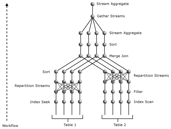
The parallel plan contains three parallelism operators. Both the Index Seek operator of the o_datkey_ptr index and the Index Scan operator of the l_order_dates_idx index are performed in parallel. This process produces several exclusive streams, which can be determined from the nearest Parallelism operators above the Index Scan, and Index Seek operators, respectively. Both operators are repartitioning the type of exchange. They reshuffle data among the streams and produce the same number of streams on their output as they have on their input. This number of streams is equal to the degree of parallelism.

The parallelism operator above the l_order_dates_idx Index Scan operator repartitions its input streams using the value of L_ORDERKEY as a key. In this way, the same values of L_ORDERKEY end up in the same output stream. At the same time, output streams maintain the order on the L_ORDERKEY column to meet the input requirement of the Merge Join operator.

The parallelism operator above the Index Seek operator repartitions its input streams using the value of O_ORDERKEY. Because its input isn't sorted on the O_ORDERKEY column values and this column is the join column in the Merge Join operator, the Sort operator between the parallelism and Merge Join operators makes sure that the input is sorted for the Merge Join operator on the join columns. The Sort operator, like the Merge Join operator, is performed in parallel.

The topmost parallelism operator gathers results from several streams into a single stream. Partial aggregations performed by the Stream Aggregate operator below the parallelism operator are then accumulated into a single SUM value for each different value of the O_ORDERPRIORITY in the Stream Aggregate operator above the parallelism operator. Because this plan has two exchange segments, with degree of parallelism equal to 4, it uses eight worker threads.

For more information about the operators used in this example, see the Logical and physical showplan operator reference.

Parallel index operations

Query plans for index operations that create or rebuild an index, or drop a clustered index, can support parallel, multithreaded operations on computers that have multiple processors.

Note

Parallel index operations are only available in Enterprise edition.

Database Engine uses the same algorithms to determine the degree of parallelism (the total number of separate worker threads to run) for index operations as it does for other queries. The max degree of parallelism server configuration option sets the maximum degree of parallelism for an index operation. You can override the max degree of parallelism value for individual index operations by setting the MAXDOP index option in the CREATE INDEX, ALTER INDEX, DROP INDEX, and ALTER TABLE statements.

When the SQL Server Database Engine builds an index execution plan, the number of parallel operations is set to the lowest value from among these values:

• The number of processors, or CPUs, in the computer.
• The number specified in the max degree of parallelism server configuration option.
• The number of CPUs that aren't already over a threshold of work performed for SQL Server worker threads.

For example, on a computer that has eight CPUs, but where max degree of parallelism is set to 6, the index operation uses no more than six parallel worker threads. If five of the CPUs in the computer exceed the threshold of SQL Server work when an index execution plan is built, the execution plan specifies only three parallel worker threads.

The main phases of a parallel index operation include:

• A coordinating worker thread quickly and randomly scans the table to estimate the distribution of the index keys. The coordinating worker thread establishes the key boundaries that create a number of key ranges equal to the degree of parallel operations, where each key range is estimated to cover similar numbers of rows. For example, if there are four million rows in the table and the degree of parallelism is 4, the coordinating worker thread determines the key values that delimit four sets of rows with 1 million rows in each set. If the coordinating worker thread can't establish enough key ranges to use all CPUs, it reduces the degree of parallelism accordingly.
• The coordinating worker thread dispatches a number of worker threads equal to the degree of parallel operations and waits for these worker threads to complete their work. Each worker thread scans the base table using a filter that retrieves only rows with key values within the range assigned to the worker thread. Each worker thread builds an index structure for the rows in its key range. In the case of a partitioned index, each worker thread builds a specified number of partitions. Partitions aren't shared among worker threads.
• After all the parallel worker threads complete, the coordinating worker thread connects the index subunits into a single index. This phase applies only to offline index operations.

Individual CREATE TABLE or ALTER TABLE statements can have multiple constraints that require creating an index. These multiple index creation operations are performed in series, although each individual index creation operation might be a parallel operation on a computer that has multiple CPUs.

Distributed query architecture

The Database Engine supports two methods for referencing heterogeneous OLE DB data sources in T-SQL statements:

• Linked server names

  Use the system stored procedures sp_addlinkedserver and sp_addlinkedsrvlogin to give a server name to an OLE DB data source. You can reference objects in these linked servers in T-SQL statements with four-part names. For example, if a linked server name of DeptSQLSrvr is defined against another instance of SQL Server, the following statement references a table on that server:

  SELECT JobTitle,
         HireDate
  FROM DeptSQLSrvr.AdventureWorks2025.HumanResources.Employee;
  

  You can also specify the linked server name in an OPENQUERY statement to open a rowset from the OLE DB data source. You can then reference this rowset like a table in T-SQL statements.

• Ad hoc connector names

  For infrequent references to a data source, specify the OPENROWSET or OPENDATASOURCE functions with the information needed to connect to the linked server. You can then reference the rowset the same way you reference a table in T-SQL statements:

  SELECT a.*
  FROM OPENROWSET (
      'Microsoft.Jet.OLEDB.4.0',
      'MSOffice\Access\Samples\Northwind.mdb';
      'Admin';
      '',
      Employees
  ) AS a;
  

The Database Engine uses OLE DB to communicate between the relational engine and the storage engine. The relational engine breaks down each T-SQL statement into a series of operations on basic OLE DB rowsets that the storage engine opens from the base tables. This process means the relational engine can also open basic OLE DB rowsets on any OLE DB data source.

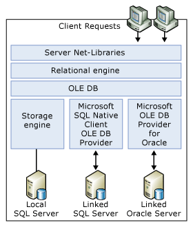
The relational engine uses the OLE DB application programming interface (API) to open the rowsets on linked servers, fetch the rows, and manage transactions.

For each OLE DB data source you access as a linked server, the server running SQL Server must have an OLE DB provider. The set of T-SQL operations that you can use against a specific OLE DB data source depends on the capabilities of the OLE DB provider.

For each instance of SQL Server, members of the sysadmin fixed server role can enable or disable the use of ad hoc connector names for an OLE DB provider by using the SQL Server DisallowAdhocAccess property. When you enable ad hoc access, any user logged on to that instance can execute T-SQL statements containing ad hoc connector names, referencing any data source on the network that the OLE DB provider can access. To control access to data sources, members of the sysadmin fixed server role can disable ad hoc access for that OLE DB provider, thereby limiting users to only those data sources referenced by linked server names defined by the administrators. By default, ad hoc access is enabled for the SQL Server OLE DB provider, and disabled for all other OLE DB providers.

Distributed queries can allow users to access another data source (for example, files, non-relational data sources such as Active Directory, and so on) by using the security context of the Windows account under which the SQL Server service is running. SQL Server impersonates the login appropriately for Windows logins. However, that impersonation isn't possible for SQL Server logins. This limitation can potentially allow a distributed query user to access another data source for which they don't have permissions, but the account under which the SQL Server service is running does have permissions. Use sp_addlinkedsrvlogin to define the specific logins that are authorized to access the corresponding linked server. This control isn't available for ad hoc names, so use caution when enabling an OLE DB provider for ad hoc access.

When possible, the Database Engine pushes relational operations such as joins, restrictions, projections, sorts, and group by operations to the OLE DB data source. The Database Engine doesn't default to scanning the base table into SQL Server and performing the relational operations itself. The Database Engine queries the OLE DB provider to determine the level of SQL grammar it supports, and, based on that information, pushes as many relational operations as possible to the provider.

The Database Engine specifies a mechanism for an OLE DB provider to return statistics indicating how key values are distributed within the OLE DB data source. This mechanism lets the Database Engine Query Optimizer better analyze the pattern of data in the data source against the requirements of each T-SQL statement, increasing the ability of the Query Optimizer to generate optimal execution plans.

Query processing on partitioned tables and indexes

The Database Engine supports partition-aware query processing for partitioned tables and indexes. This section describes how the query processor handles partitioned objects, how to interpret execution plans that involve partitioning, and best practices for improving query performance on partitioned objects.

Note

Partitioned tables and indexes are supported in SQL Server Standard edition, starting with SQL Server 2016 (13.x) with Service Pack 1.

New partition-aware seek operation

In the Database Engine, the query processor internally sees a partitioned table as a multicolumn index with PartitionID as the leading column. PartitionID is a hidden computed column used internally to represent the ID of the partition containing a specific row. For example, assume the table T, defined as T(a, b, c), is partitioned on column a, and has a clustered index on column b. This partitioned table is treated as a nonpartitioned table with the schema T(PartitionID, a, b, c) and a clustered index on the composite key (PartitionID, b). This representation enables the Query Optimizer to perform seek operations based on PartitionID on any partitioned table or index.

Partition elimination is now done in this seek operation.

In addition, the Query Optimizer is extended so that a seek or scan operation with one condition can be done on PartitionID (as the logical leading column) and possibly other index key columns. The query processor then performs a second-level seek, with a different condition, on one or more additional columns, for each distinct value that meets the qualification for the first-level seek operation. This operation, called a partition skip scan, allows the Query Optimizer to perform a seek or scan operation based on one condition to determine the partitions to access, and a second-level index seek operation within that operator to return rows from these partitions that meet a different condition. For example, consider the following query.

SELECT *
FROM T
WHERE a < 10
      AND b = 2;

For this example, assume that table T, defined as T(a, b, c), is partitioned on column a, and has a clustered index on column b. The following partition function defines the partition boundaries for table T:

CREATE PARTITION FUNCTION myRangePF1(INT)
    AS RANGE LEFT
    FOR VALUES (3, 7, 10);

To solve the query, the query processor performs a first-level seek operation to find every partition that contains rows that meet the condition T.a < 10. This operation identifies the partitions to access. Within each partition identified, the processor then performs a second-level seek into the clustered index on column b to find the rows that meet the condition T.b = 2 and T.a < 10.

The following illustration is a logical representation of the partition skip scan operation. It shows table T with data in columns a and b. The partitions are numbered 1 through 4 with the partition boundaries shown by dashed vertical lines. A first-level seek operation to the partitions (not shown in the illustration) determines that partitions 1, 2, and 3 meet the seek condition implied by the partitioning defined for the table and the predicate on column a (T.a < 10). The path traversed by the second-level seek is illustrated by the curved line. Essentially, the operation seeks into each of these partitions for rows that meet the condition b = 2. The total cost of the operation is the same as that of three separate index seeks.

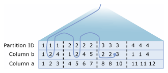
Display partitioning information in query execution plans

Examine the execution plans of queries on partitioned tables and indexes by using the T-SQL SET statements SET SHOWPLAN_XML or SET STATISTICS XML, or by using the graphical execution plan output in SSMS. For example, you can display the compile-time execution plan by selecting Display Estimated Execution Plan on the Query Editor toolbar and the run-time plan by selecting Include Actual Execution Plan.

By using these tools, you can find the following information:

• The operations such as scans, seeks, inserts, updates, merges, and deletes that access partitioned tables or indexes.
• The partitions accessed by the query. For example, run-time execution plans include the total count of partitions accessed and the ranges of contiguous partitions that are accessed.
• When a partition skip scan operation is used in a seek or scan operation to retrieve data from one or more partitions.

Partition information enhancements

The Database Engine provides enhanced partitioning information for both compile-time and run-time execution plans. Execution plans now provide the following information:

• An optional Partitioned attribute that indicates that an operator, such as a seek, scan, insert, update, merge, or delete, is performed on a partitioned table.
• A new SeekPredicateNew element with a SeekKeys subelement that includes PartitionID as the leading index key column and filter conditions that specify range seeks on PartitionID. The presence of two SeekKeys subelements indicates a partition skip scan on PartitionID.
• Summary information that provides a total count of the partitions accessed. This information is available only in run-time plans.

To demonstrate how this information is displayed in both the graphical execution plan output and the XML Showplan output, consider the following query on the partitioned table fact_sales. This query updates data in two partitions.

UPDATE fact_sales
    SET quantity = quantity - 2
WHERE date_id BETWEEN 20190802 AND 20190902;

The following illustration shows the properties of the Clustered Index Seek operator in the runtime execution plan for this query. To view the definition of the fact_sales table and the partition definition, see Example.

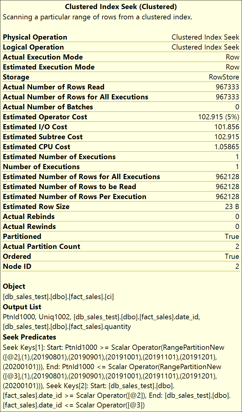
Partitioned attribute

When an operator such as an Index Seek is executed on a partitioned table or index, the Partitioned attribute appears in the compile-time and run-time plan, and is set to True (1). The attribute doesn't display when it's set to False (0).

The Partitioned attribute can appear in the following physical and logical operators:

• Table Scan
• Index Scan
• Index Seek
• Insert
• Update
• Delete
• Merge

As shown in the previous illustration, this attribute appears in the properties of the operator in which it's defined. In the XML Showplan output, this attribute appears as Partitioned="1" in the RelOp node of the operator in which it's defined.

New seek predicate

In XML Showplan output, the SeekPredicateNew element appears in the operator in which it's defined. It can contain up to two occurrences of the SeekKeys subelement. The first SeekKeys item specifies the first-level seek operation at the partition ID level of the logical index. That is, this seek operation determines the partitions that must be accessed to satisfy the conditions of the query. The second SeekKeys item specifies the second-level seek that occurs within each partition identified in the first-level seek.

Partition summary information

In run-time execution plans, partition summary information provides a count of the partitions accessed and the identity of the actual partitions accessed. You can use this information to verify that the correct partitions are accessed in the query and that all other partitions are eliminated from consideration.

The following information is provided: Actual Partition Count, and Partitions Accessed.

Actual Partition Count is the total number of partitions accessed by the query.

Partitions Accessed, in XML Showplan output, is the partition summary information that appears in the new RuntimePartitionSummary element in RelOp node of the operator in which it's defined. The following example shows the contents of the RuntimePartitionSummary element, indicating that two total partitions are accessed (partitions 2 and 3).

<RunTimePartitionSummary>
    <PartitionsAccessed PartitionCount="2" >
        <PartitionRange Start="2" End="3" />
    </PartitionsAccessed>
</RunTimePartitionSummary>

Display partition information by using other showplan methods

The Showplan methods SHOWPLAN_ALL, SHOWPLAN_TEXT, and STATISTICS PROFILE don't report the partition information described in this article, with the following exception. As part of the SEEK predicate, the partitions to be accessed are identified by a range predicate on the computed column representing the partition ID. The following example shows the SEEK predicate for a Clustered Index Seek operator. Partitions 2 and 3 are accessed, and the seek operator filters on the rows that meet the condition date_id BETWEEN 20190802 AND 20190902.

|--Clustered Index Seek(OBJECT:([db_sales_test].[dbo].[fact_sales].[ci]),
        SEEK:([PtnId1000] >= (2) AND [PtnId1000] <= (3)
                AND [db_sales_test].[dbo].[fact_sales].[date_id] >= (20190802)
                AND [db_sales_test].[dbo].[fact_sales].[date_id] <= (20190902))
                ORDERED FORWARD)

Interpret execution plans for partitioned heaps

A partitioned heap is treated as a logical index on the partition ID. In an execution plan, partition elimination on a partitioned heap is represented as a Table Scan operator with a SEEK predicate on partition ID. The following example shows the Showplan information provided:

|-- Table Scan (OBJECT: ([db].[dbo].[T]), SEEK: ([PtnId1001]=[Expr1011]) ORDERED FORWARD)

Interpret execution plans for collocated joins

Join collocation can occur when two tables are partitioned using the same or equivalent partitioning function and the partitioning columns from both sides of the join are specified in the join condition of the query. The Query Optimizer can generate a plan where the partitions of each table that have equal partition IDs are joined separately. Collocated joins can be faster than non-collocated joins because they can require less memory and processing time. The Query Optimizer chooses a non-collocated plan or a collocated plan based on cost estimates.

In a collocated plan, the Nested Loops join reads one or more joined table or index partitions from the inner side. The numbers within the Constant Scan operators represent the partition numbers.

When parallel plans for collocated joins are generated for partitioned tables or indexes, a Parallelism operator appears between the Constant Scan and the Nested Loops join operators. In this case, multiple worker threads on the outer side of the join each read and work on a different partition.

The following illustration demonstrates a parallel query plan for a collocated join.

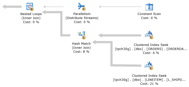
Parallel query execution strategy for partitioned objects

The query processor uses a parallel execution strategy for queries that select from partitioned objects. As part of the execution strategy, the query processor determines the table partitions required for the query, and the proportion of worker threads to allocate to each partition. In most cases, the query processor allocates an equal or almost equal number of worker threads to each partition, and then executes the query in parallel across the partitions. The following paragraphs explain worker thread allocation in greater detail.

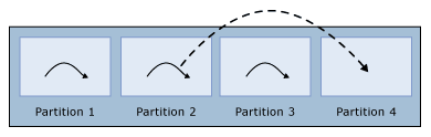
If the number of worker threads is less than the number of partitions, the query processor assigns each worker thread to a different partition, initially leaving one or more partitions without an assigned worker thread. When a worker thread finishes executing on a partition, the query processor assigns it to the next partition until each partition is assigned a single worker thread. This assignment is the only case in which the query processor reallocates worker threads to other partitions.

Shows worker thread reassigned after it finishes. If the number of worker threads is equal to the number of partitions, the query processor assigns one worker thread to each partition. When a worker thread finishes, it isn't reallocated to another partition.

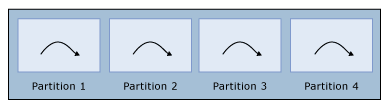
If the number of worker threads is greater than the number of partitions, the query processor allocates an equal number of worker threads to each partition. If the number of worker threads isn't an exact multiple of the number of partitions, the query processor allocates one extra worker thread to some partitions in order to use all of the available worker threads. If there's only one partition, all worker threads are assigned to that partition. In the following diagram, there are four partitions and 14 worker threads. Each partition has three worker threads assigned, and two partitions have an extra worker thread, for a total of 14 worker thread assignments. When a worker thread finishes, it isn't reassigned to another partition.

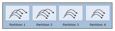
Although the previous examples suggest a straightforward way to allocate worker threads, the actual strategy is more complex and accounts for other variables that occur during query execution. For example, if the table is partitioned and has a clustered index on column A and a query has the predicate clause WHERE A IN (13, 17, 25), the query processor allocates one or more worker threads to each of these three seek values (A = 13, A = 17, and A = 25) instead of each table partition. It's only necessary to execute the query in the partitions that contain these values, and if all of these seek predicates happen to be in the same table partition, all worker threads are assigned to the same table partition.

To take another example, suppose that the table has four partitions on column A with boundary points (10, 20, 30), an index on column B, and the query has a predicate clause WHERE B IN (50, 100, 150). Because the table partitions are based on the values of A, the values of B can occur in any of the table partitions. Thus, the query processor seeks for each of the three values of B (50, 100, 150) in each of the four table partitions. The query processor assigns worker threads proportionately so that it can execute each of these 12 query scans in parallel.

Table partitions based on column A	Seeks for column B in each table partition
Table Partition 1: A < 10	B = 50, B = 100, B = 150
Table Partition 2: A >= 10 AND A < 20	B = 50, B = 100, B = 150
Table Partition 3: A >= 20 AND A < 30	B = 50, B = 100, B = 150
Table Partition 4: A >= 30	B = 50, B = 100, B = 150

Best practices

To improve the performance of queries that access a large amount of data from large partitioned tables and indexes, follow these best practices:

• Stripe each partition across many disks. This approach is especially relevant when using spinning disks.

• When possible, use a server with enough main memory to fit frequently accessed partitions, or all partitions in memory, to reduce I/O cost.

• If the data you query doesn't fit in memory, compress the tables and indexes to reduce I/O cost.

• Use a server with fast processors and as many processor cores as you can afford, to take advantage of parallel query processing capability.

• Ensure the server has sufficient I/O controller bandwidth.

• Create a clustered index on every large partitioned table to take advantage of B-tree scanning optimizations.

• When bulk loading data into partitioned tables, follow the best practice recommendations in the white paper, The Data Loading Performance Guide.

Example

The following example creates a test database containing a single table with seven partitions. To view partitioning information for both compile-time and run-time plans, use the tools described in Display partitioning information in query execution plans when executing the queries in this example.

Note

This example inserts more than 1 million rows into the table. Running this example can take several minutes depending on your hardware. Before executing this example, verify that you have more than 1.5 GB of disk space available.

USE master;
GO

IF DB_ID(N'db_sales_test') IS NOT NULL
    DROP DATABASE db_sales_test;
GO

CREATE DATABASE db_sales_test;
GO

USE db_sales_test;
GO

CREATE PARTITION FUNCTION pf_range_fact(INT)
    AS RANGE RIGHT
    FOR VALUES (20190801, 20190901, 20191001, 20191101, 20191201, 20200101);
GO

CREATE PARTITION SCHEME ps_fact_sales
    AS PARTITION pf_range_fact
    ALL TO ([PRIMARY]);
GO

CREATE TABLE fact_sales
(
    date_id INT,
    product_id INT,
    store_id INT,
    quantity INT,
    unit_price NUMERIC (7, 2),
    other_data CHAR (1000)
) ON ps_fact_sales (date_id);
GO

CREATE CLUSTERED INDEX ci
    ON fact_sales(date_id);
GO

PRINT 'Loading...';

SET NOCOUNT ON;

DECLARE @i AS INT;

SET @i = 1;

WHILE (@i < 1000000)
    BEGIN
        INSERT INTO fact_sales
        VALUES (20190800 + (@i % 30) + 1, @i % 10000, @i % 200, RAND() - 25, (@i % 3) + 1, '');
        SET @i += 1;
    END
GO

DECLARE @i AS INT;

SET @i = 1;

WHILE (@i < 10000)
    BEGIN
        INSERT INTO fact_sales
        VALUES (20190900 + (@i % 30) + 1, @i % 10000, @i % 200, RAND() - 25, (@i % 3) + 1, '');
        SET @i += 1;
    END

PRINT 'Done.';
GO

-- Two-partition query.
SET STATISTICS XML ON;
GO

SELECT date_id,
       SUM(quantity * unit_price) AS total_price
FROM fact_sales
WHERE date_id BETWEEN 20190802 AND 20190902
GROUP BY date_id;
GO

SET STATISTICS XML OFF;
GO

-- Single-partition query.
SET STATISTICS XML ON;
GO

SELECT date_id,
       SUM(quantity * unit_price) AS total_price
FROM fact_sales
WHERE date_id BETWEEN 20190801 AND 20190831
GROUP BY date_id;
GO

SET STATISTICS XML OFF;
GO

Related content

• Logical and physical showplan operator reference
• Extended Events overview
• Best practices for monitoring workloads with Query Store
• Cardinality Estimation (SQL Server)
• Intelligent query processing in SQL databases
• Operator precedence (Transact-SQL)
• Execution plan overview
• Performance Center for SQL Server Database Engine and Azure SQL Database