Note
Access to this page requires authorization. You can try signing in or changing directories.
Access to this page requires authorization. You can try changing directories.
In this quickstart, you learn how to use the Microsoft Quantum resource estimator to estimate the resources of a Q# program.
Prerequisites
- The latest version of Visual Studio Code (VS Code) or open VS Code for the Web.
- The latest version of the Microsoft Quantum Development Kit (QDK) extension. For installation details, see Set up the QDK extension.
Tip
You don't need to have an Azure account to run the resource estimator.
Load a Q# sample program
- In VS Code, open the File menu and choose New File.
- Save the file as RandomNum.qs.
- To open the menu of Q# samples, open RandomNum.qs and enter
sample. - Choose Random Bits sample and save the file again.
Run the resource estimator
The resource estimator offers six predefined qubit parameters, four of which have gate-based instruction sets and two that have a Majorana instruction set. The resource estimator also offers two quantum error correction codes, surface_code and floquet_code.
In this example, you run the resource estimator with the qubit_gate_us_e3 qubit parameter and the surface_code quantum error correction code.
- In VS Code, open the View menu and choose Command Palette.
- Enter and select QDK: Calculate Resource Estimates. The Qubit types menu appears where you can select one or more qubit parameters.
- For this example, select only qubit_gate_us_e3, and then choose the OK button.
- In the Error budget menu, enter 0.001.
- In the Friendly name for run menu, press Enter to accept the default run name, which is based on the Q# filename RandomNum.qs.
A new QDK Estimates tab opens with the resource estimator results for your random bit program.
View the resource estimator results
The resource estimator provides multiple estimates for the same algorithm. Compare the estimates to understand the tradeoffs between the number of qubits and the runtime. To view the results and compare estimates, follow these steps:
Go to the QDK Estimates tab.
The Results dropdown displays a summary of the resource estimation. Choose the menu icon in the first row to select the columns that display. For example, select Estimate type, Qubit type, Logical qubits, T factory fraction, Runtime, and Physical qubits.
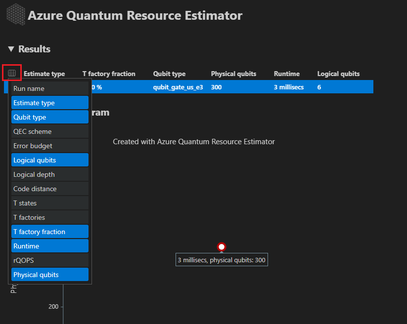
The number of optimal combinations of {number of qubits, runtime} for your algorithm is in the Estimate type column of the results table. Each combination appears as a point in the space-time diagram. In this case, there's only one combination.
Note
If you select more than one qubit parameter and error correction code in the configuration, then the results display in different rows for each selection. Choose a result row from the table to bring up the corresponding space-time diagram and report data.
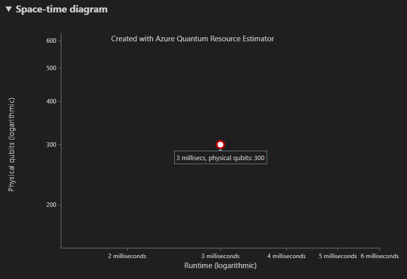
The Space-time diagram dropdown shows the tradeoffs between the number of physical qubits and the runtime of the algorithm. In this case, the resource estimator finds one optimal combination out of many thousands of possible combinations. To view an estimation summary for a combination, hover over or select the corresponding point in the diagram. For more information, see Space-time diagram.
Note
Select a point in the space-time diagram to see the space diagram and the details of the resource estimation that correspond to that point.
The Space diagram dropdown displays the distribution of physical qubits that your algorithm uses and the T factories. In this example, the algorithm qubits and the total qubits are the same because the algorithm doesn't use any T factory copies.
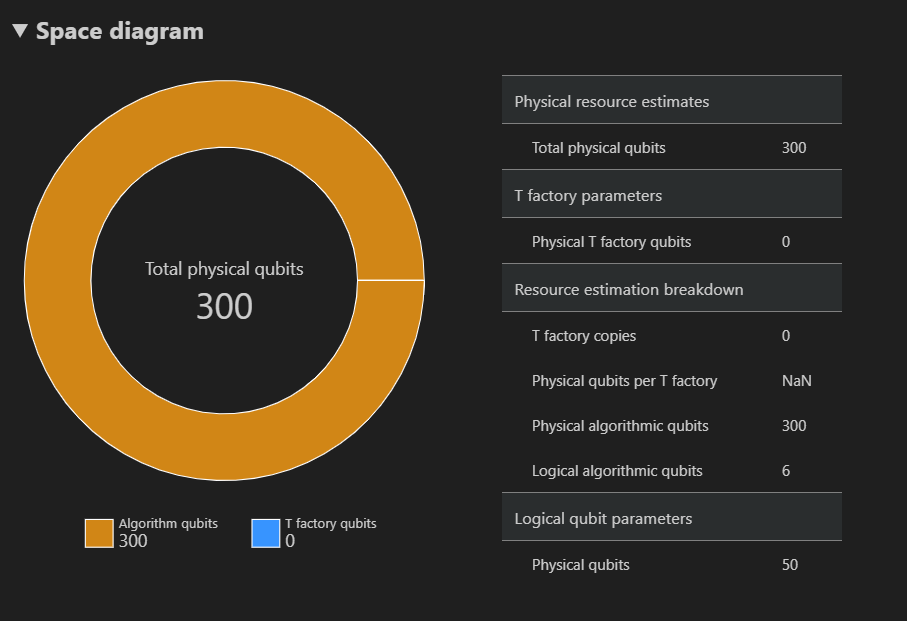
The Resource Estimates dropdown displays the full list of output data from the resource estimator. To view more information about each resource category, expand the corresponding dropdown. For example, expand the Logical qubit parameters group.
Logical qubit parameter Value QEC scheme surface_codeCode distance 5 Physical qubits 50 Logical cycle time 3 millisecs Logical qubit error rate 3.00e-5 Crossing prefactor 0.03 Error correction threshold 0.01 Logical cycle time formula (4 * twoQubitGateTime+ 2 *oneQubitMeasurementTime) *codeDistancePhysical qubits formula 2 * codeDistance*codeDistanceTip
Click Show detailed rows to display the description of each output of the report data.
For more information, see Retrieve the output of the Microsoft Quantum resource estimator for the resource estimator.
The full functionality of the resource estimator is beyond the scope of this quickstart. For more information, see Different ways to run the Microsoft Quantum resource estimator.
Note
If you have issues when you work with the resource estimator, then see the Troubleshooting page, or contact AzureQuantumInfo@microsoft.com.