Lakehouse tutorial: Prepare and transform data in the lakehouse

In this tutorial, you use notebooks with Spark runtime to transform and prepare raw data in your lakehouse.

Prerequisites

Before you begin, you must complete the previous tutorials in this series:

1. Create a lakehouse
2. Ingest data into the lakehouse

Prepare data

From the previous tutorial steps, you have raw data ingested from the source to the Files section of the lakehouse. Now you can transform that data and prepare it for creating Delta tables.

1. Download the notebooks from the Lakehouse Tutorial Source Code folder.

2. In your browser, go to your Fabric workspace in the Fabric portal.

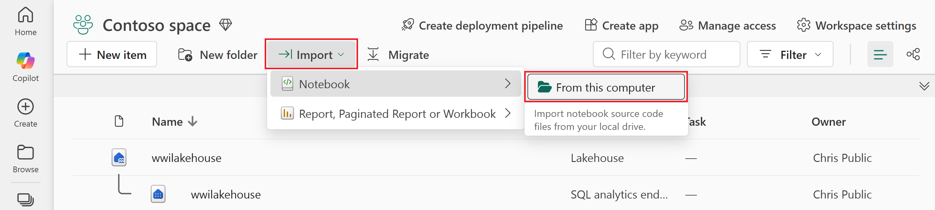
3. Select Import > Notebook > From this computer.

   

4. Select Upload from the Import status pane that opens on the right side of the screen.

5. Select all the notebooks that you downloaded in the first step of this section.

   

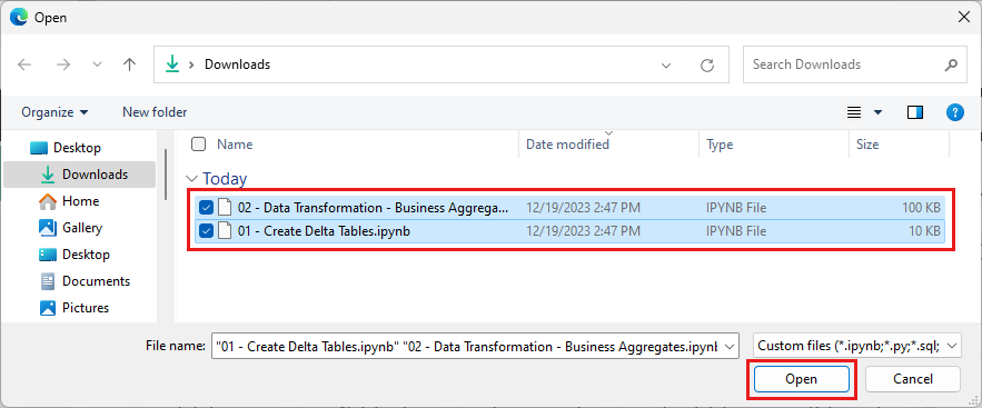
6. Select Open. A notification indicating the status of the import appears in the top right corner of the browser window.

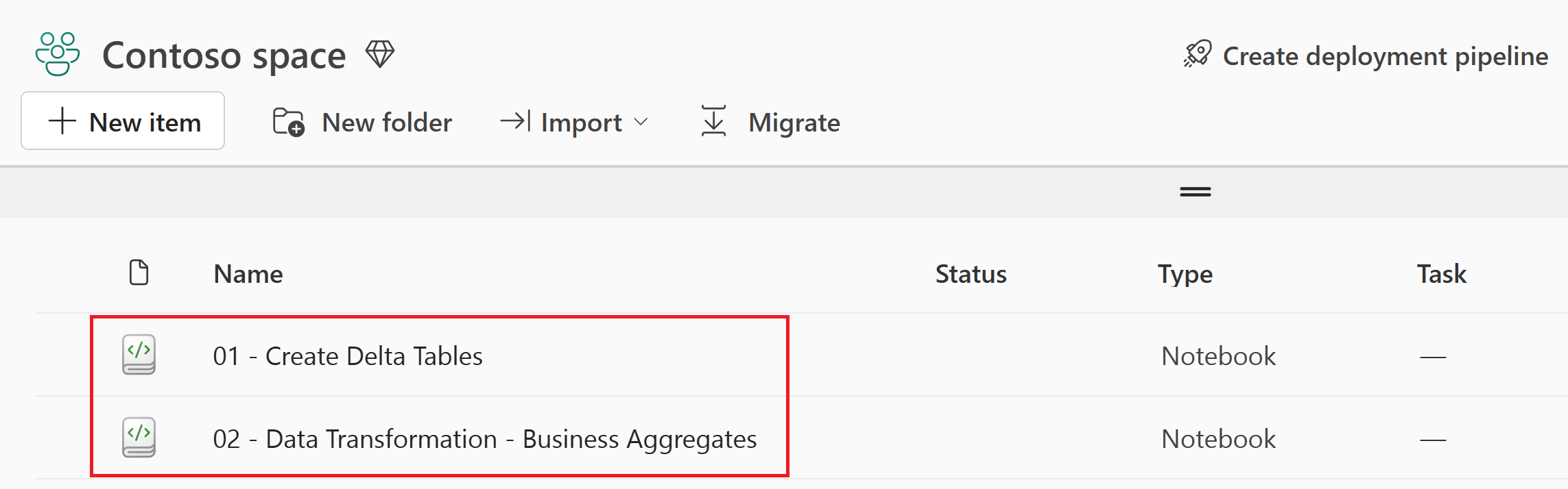
7. After the import is successful, go to the items view of the workspace to verify the newly imported notebooks.

   

Create Delta tables

In this section, you open the 01 - Create Delta Tables notebook and run through each cell to create Delta tables from the raw data. The tables follow a star schema, which is a common pattern for organizing analytical data:

• A fact table (fact_sale) contains the measurable events of the business — in this case, individual sales transactions with quantities, prices, and profit.
• Dimension tables (dimension_city, dimension_customer, dimension_date, dimension_employee, dimension_stock_item) contain the descriptive attributes that give context to the facts, such as where a sale happened, who made it, and when.

1. Select the wwilakehouse lakehouse to open it, so that the notebook you open next is linked to it.

2. From the top navigation menu, select Open notebook > Existing notebook.

   

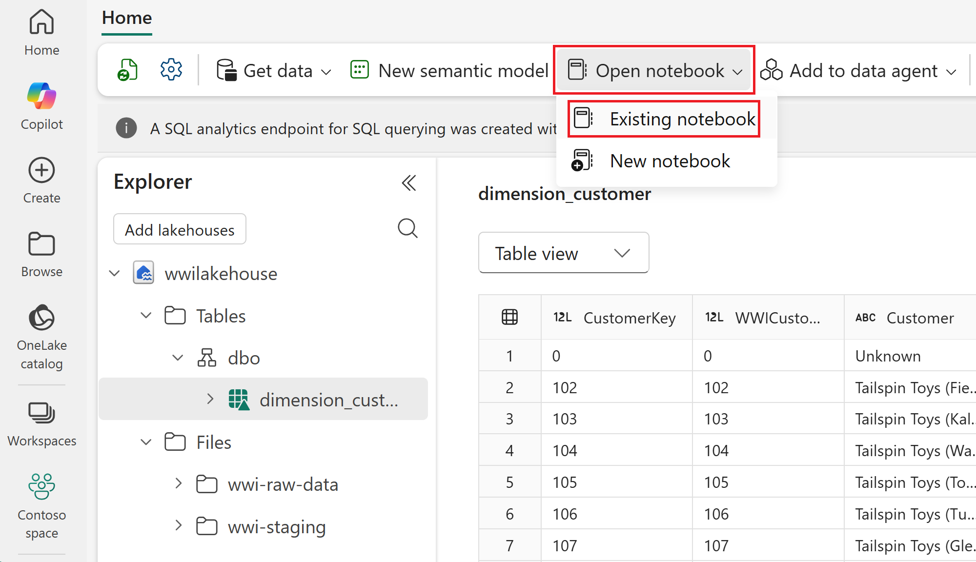
3. Select the 01 - Create Delta Tables notebook and select Open. The notebook is already linked to your opened lakehouse, as shown in the lakehouse Explorer.

   Note

   In the following steps, you run each cell in the notebook sequentially. To execute a cell, select the Run icon that appears to the left of the cell upon hover, or press SHIFT + ENTER on your keyboard while the cell is selected. Alternatively, you can select Run all on the top ribbon (under Home) to execute all cells in sequence.

4. Cell 1 - Spark session configuration. This cell enables two Fabric features that optimize how data is written and read in subsequent cells. V-order optimizes the parquet file layout for faster reads and better compression. Optimize write reduces the number of files written and increases individual file size.

   Run this cell.

   spark.conf.set("spark.sql.parquet.vorder.enabled", "true")
   spark.conf.set("spark.microsoft.delta.optimizeWrite.enabled", "true")
   spark.conf.set("spark.microsoft.delta.optimizeWrite.binSize", "1073741824")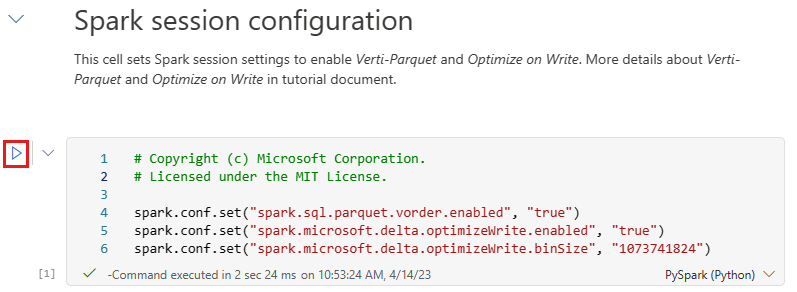
   

   

   Tip

   You don't need to specify any Spark pool or cluster details. Fabric provides a default Spark pool called Live Pool for every workspace. When you execute the first cell, the live pool starts in a few seconds and establishes the Spark session. Subsequent cells run almost instantaneously while the session is active.

5. Cell 2 - Fact - Sale. This cell reads raw parquet data from the wwi-raw-data folder, which was ingested into the lakehouse in the previous tutorial. It adds date part columns (Year, Quarter, and Month), then writes the data as a Delta table partitioned by Year and Quarter. Partitioning organizes the data into subdirectories, which improves query performance when filtering by these columns.

   Run this cell.

   from pyspark.sql.functions import col, year, month, quarter
   
   table_name = 'fact_sale'
   
   df = spark.read.format("parquet").load('Files/wwi-raw-data/full/fact_sale_1y_full')
   df = df.withColumn('Year', year(col("InvoiceDateKey")))
   df = df.withColumn('Quarter', quarter(col("InvoiceDateKey")))
   df = df.withColumn('Month', month(col("InvoiceDateKey")))
   
   df.write.mode("overwrite").format("delta").partitionBy("Year","Quarter").save("Tables/" + table_name)
   

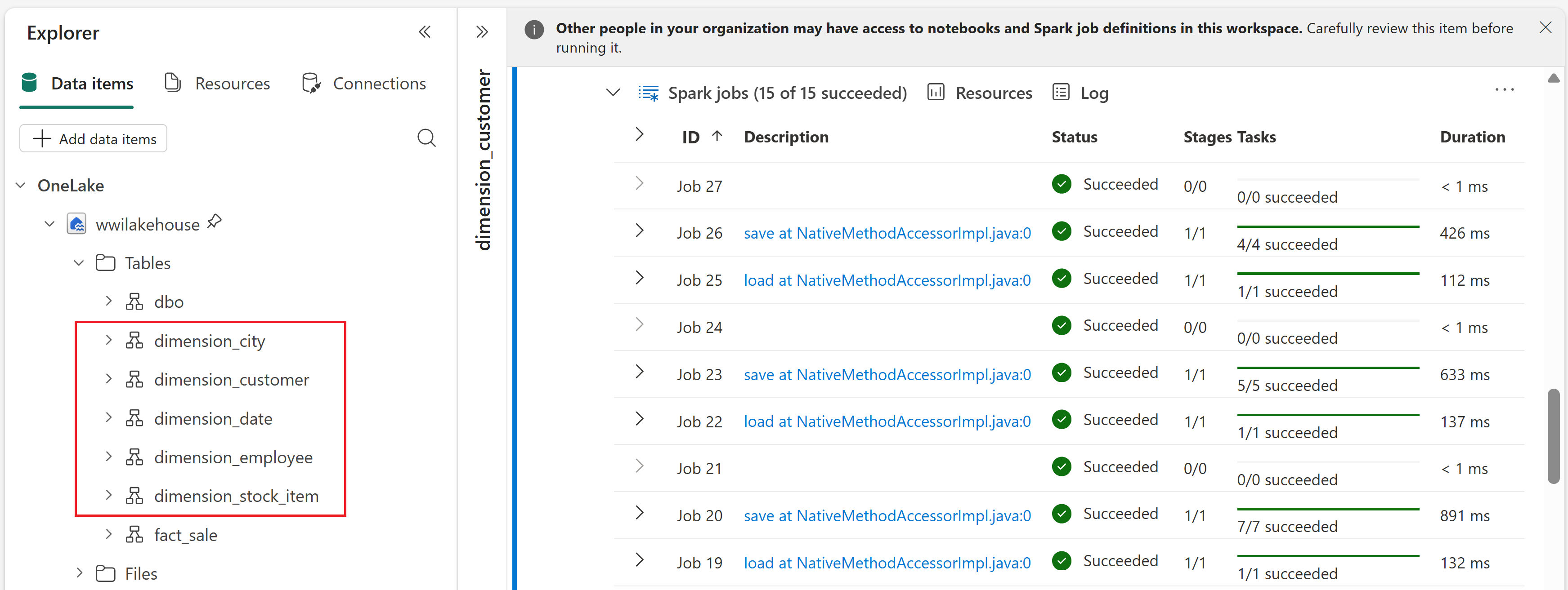
6. Cell 3 - Dimensions. This cell loads the dimension tables that provide descriptive context for the fact table, such as cities, customers, and dates. It defines a function that reads raw parquet data from the wwi-raw-data folder for a given table name, drops the unused Photo column, and writes each table as a Delta table. It then loops through five dimension tables (dimension_city, dimension_customer, dimension_date, dimension_employee, and dimension_stock_item) and creates a Delta table for each one.

   Run this cell.

   from pyspark.sql.types import *
   def loadFullDataFromSource(table_name):
       df = spark.read.format("parquet").load('Files/wwi-raw-data/full/' + table_name)
       df = df.drop("Photo")
       df.write.mode("overwrite").format("delta").save("Tables/" + table_name)
   
   full_tables = [
       'dimension_city',
       'dimension_customer',
       'dimension_date',
       'dimension_employee',
       'dimension_stock_item'
       ]
   
   for table in full_tables:
       loadFullDataFromSource(table)
   

7. To validate the created tables, right-click the wwilakehouse lakehouse in the explorer and then select Refresh. The tables appear.

   

Transform data for business aggregates

In this section, you open the 02 - Data Transformation - Business Aggregates notebook and run through each cell to create aggregate tables from the Delta tables you created in the previous section.

1. Select the wwilakehouse lakehouse to open it again, so that the notebook you open next is linked to it.

2. From the top navigation menu, select Open notebook > Existing notebook. Select the 02 - Data Transformation - Business Aggregates notebook and select Open.

   This notebook uses two different coding approaches to create two aggregate tables. You run all the cells—each approach creates a different table:

   • Approach #1 uses PySpark to create the aggregate_sale_by_date_city table. This approach is preferable if you have a Python or PySpark background.
   • Approach #2 uses Spark SQL to create the aggregate_sale_by_date_employee table. This approach is preferable if you have a SQL background.

   In the following steps, you run each cell in the notebook sequentially, just as you did in the previous section.

3. Cell 1 - Spark session configuration. As in the previous notebook, this cell enables V-order and Optimize Write for the Spark session.

   Run this cell.

   spark.conf.set("spark.sql.parquet.vorder.enabled", "true")
   spark.conf.set("spark.microsoft.delta.optimizeWrite.enabled", "true")
   spark.conf.set("spark.microsoft.delta.optimizeWrite.binSize", "1073741824")
   

4. Cell 2 - Approach #1 - sale_by_date_city. This cell loads the fact_sale, dimension_date, and dimension_city Delta tables into PySpark dataframes, preparing the data for joining and aggregation in the next cell.

   Run this cell.

   df_fact_sale = spark.read.table("wwilakehouse.fact_sale") 
   df_dimension_date = spark.read.table("wwilakehouse.dimension_date")
   df_dimension_city = spark.read.table("wwilakehouse.dimension_city")
   

   If you enabled lakehouse schemas on your lakehouse, replace the cell contents with the following code and run it:

   df_fact_sale = spark.read.format("delta").load("Tables/fact_sale")
   df_dimension_date = spark.read.format("delta").load("Tables/dimension_date")
   df_dimension_city = spark.read.format("delta").load("Tables/dimension_city")
   

5. Cell 3. This cell joins the three dataframes on their key columns, selects date, city, and sales fields, then groups and sums sales totals and profit by date and city. It writes the result as the aggregate_sale_by_date_city Delta table, which summarizes sales performance by geography.

   Run this cell.

   sale_by_date_city = df_fact_sale.alias("sale") \
   .join(df_dimension_date.alias("date"), df_fact_sale.InvoiceDateKey == df_dimension_date.Date, "inner") \
   .join(df_dimension_city.alias("city"), df_fact_sale.CityKey == df_dimension_city.CityKey, "inner") \
   .select("date.Date", "date.CalendarMonthLabel", "date.Day", "date.ShortMonth", "date.CalendarYear", "city.City", "city.StateProvince", "city.SalesTerritory", "sale.TotalExcludingTax", "sale.TaxAmount", "sale.TotalIncludingTax", "sale.Profit")\
   .groupBy("date.Date", "date.CalendarMonthLabel", "date.Day", "date.ShortMonth", "date.CalendarYear", "city.City", "city.StateProvince", "city.SalesTerritory")\
   .sum("sale.TotalExcludingTax", "sale.TaxAmount", "sale.TotalIncludingTax", "sale.Profit")\
   .withColumnRenamed("sum(TotalExcludingTax)", "SumOfTotalExcludingTax")\
   .withColumnRenamed("sum(TaxAmount)", "SumOfTaxAmount")\
   .withColumnRenamed("sum(TotalIncludingTax)", "SumOfTotalIncludingTax")\
   .withColumnRenamed("sum(Profit)", "SumOfProfit")\
   .orderBy("date.Date", "city.StateProvince", "city.City")
   
   sale_by_date_city.write.mode("overwrite").format("delta").option("overwriteSchema", "true").save("Tables/aggregate_sale_by_date_city")
   

6. Cell 4 - Approach #2 - sale_by_date_employee. This cell uses Spark SQL to create a temporary view called sale_by_date_employee. The query joins fact_sale, dimension_date, and dimension_employee, groups by date and employee columns, and calculates aggregated sales totals and profit, summarizing sales performance by employee.

   Run this cell.

   %%sql
   CREATE OR REPLACE TEMPORARY VIEW sale_by_date_employee
   AS
   SELECT
          DD.Date, DD.CalendarMonthLabel
    , DD.Day, DD.ShortMonth Month, CalendarYear Year
         ,DE.PreferredName, DE.Employee
         ,SUM(FS.TotalExcludingTax) SumOfTotalExcludingTax
         ,SUM(FS.TaxAmount) SumOfTaxAmount
         ,SUM(FS.TotalIncludingTax) SumOfTotalIncludingTax
         ,SUM(Profit) SumOfProfit 
   FROM wwilakehouse.fact_sale FS
   INNER JOIN wwilakehouse.dimension_date DD ON FS.InvoiceDateKey = DD.Date
   INNER JOIN wwilakehouse.dimension_Employee DE ON FS.SalespersonKey = DE.EmployeeKey
   GROUP BY DD.Date, DD.CalendarMonthLabel, DD.Day, DD.ShortMonth, DD.CalendarYear, DE.PreferredName, DE.Employee
   ORDER BY DD.Date ASC, DE.PreferredName ASC, DE.Employee ASC
   

   If you enabled lakehouse schemas, replace the cell contents with the following Spark SQL code and run it:

   %%sql
   CREATE OR REPLACE TEMPORARY VIEW sale_by_date_employee
   AS
   SELECT
          DD.Date, DD.CalendarMonthLabel
    , DD.Day, DD.ShortMonth Month, CalendarYear Year
         ,DE.PreferredName, DE.Employee
         ,SUM(FS.TotalExcludingTax) SumOfTotalExcludingTax
         ,SUM(FS.TaxAmount) SumOfTaxAmount
         ,SUM(FS.TotalIncludingTax) SumOfTotalIncludingTax
         ,SUM(Profit) SumOfProfit 
   FROM delta.`Tables/fact_sale` FS
   INNER JOIN delta.`Tables/dimension_date` DD ON FS.InvoiceDateKey = DD.Date
   INNER JOIN delta.`Tables/dimension_employee` DE ON FS.SalespersonKey = DE.EmployeeKey
   GROUP BY DD.Date, DD.CalendarMonthLabel, DD.Day, DD.ShortMonth, DD.CalendarYear, DE.PreferredName, DE.Employee
   ORDER BY DD.Date ASC, DE.PreferredName ASC, DE.Employee ASC
   

7. Cell 5. This cell reads from the sale_by_date_employee temporary view created in the previous cell and writes the results as the aggregate_sale_by_date_employee Delta table.

   Run this cell.

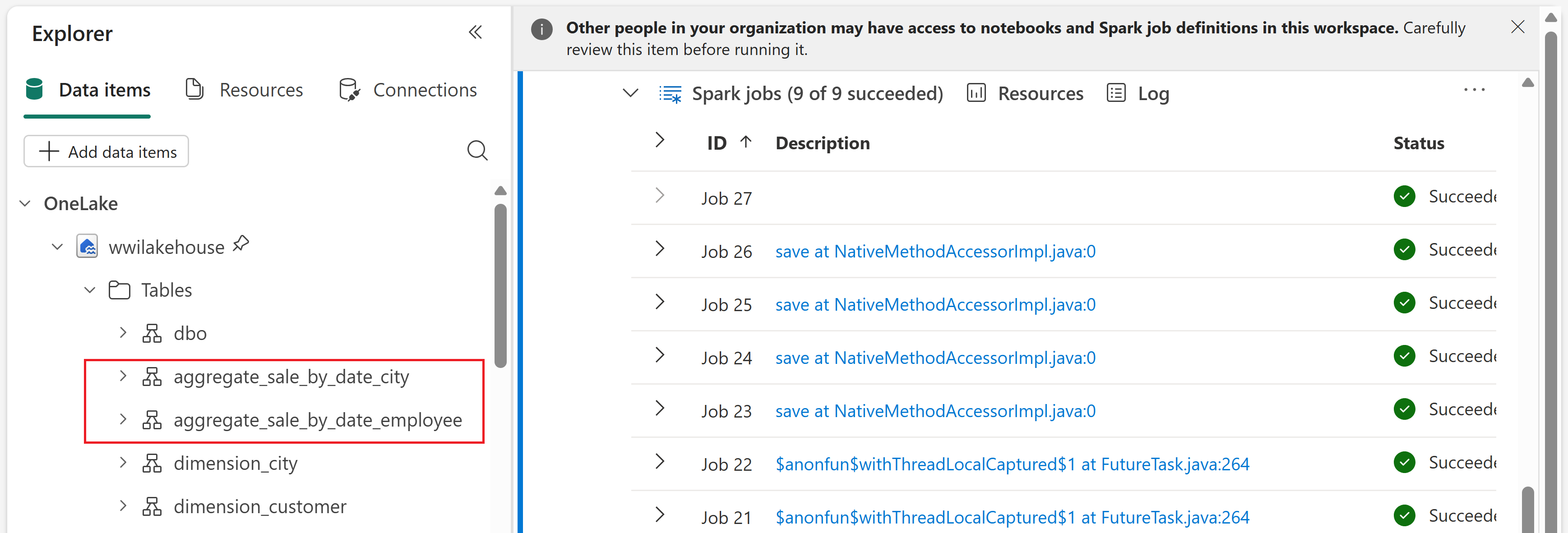
   sale_by_date_employee = spark.sql("SELECT * FROM sale_by_date_employee")
   sale_by_date_employee.write.mode("overwrite").format("delta").option("overwriteSchema", "true").save("Tables/aggregate_sale_by_date_employee")
   

8. To validate the created tables, right-click the wwilakehouse lakehouse in the explorer and then select Refresh. The aggregate tables appear.

   

Note

The data in this tutorial is written as Delta lake files. The automatic table discovery and registration feature of Fabric picks up and registers them in the metastore. You don't need to explicitly call CREATE TABLE statements to create tables to use with SQL.

Next step

Create a semantic model and build a report