הערה
הגישה לדף זה מחייבת הרשאה. באפשרותך לנסות להיכנס או לשנות מדריכי כתובות.
הגישה לדף זה מחייבת הרשאה. באפשרותך לנסות לשנות מדריכי כתובות.
In this tutorial, you'll learn how to conduct exploratory data analysis (EDA) to examine and investigate the data while summarizing its key characteristics through the use of data visualization techniques.
You'll use seaborn, a Python data visualization library that provides a high-level interface for building visuals on dataframes and arrays. For more information about seaborn, see Seaborn: Statistical Data Visualization.
You'll also use Data Wrangler, a notebook-based tool that provides you with an immersive experience to conduct exploratory data analysis and cleaning.
The main steps in this tutorial are:
- Read the data stored from a delta table in the lakehouse.
- Convert a Spark DataFrame to Pandas DataFrame, which python visualization libraries support.
- Use Data Wrangler to perform initial data cleaning and transformation.
- Perform exploratory data analysis using
seaborn.
Prerequisites
Get a Microsoft Fabric subscription. Or, sign up for a free Microsoft Fabric trial.
Sign in to Microsoft Fabric.
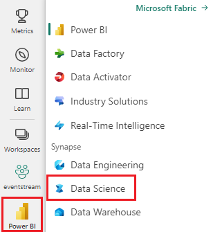
Switch to Fabric by using the experience switcher on the lower-left side of your home page.
This is part 2 of 5 in the tutorial series. To complete this tutorial, first complete:
Follow along in notebook
2-explore-cleanse-data.ipynb is the notebook that accompanies this tutorial.
To open the accompanying notebook for this tutorial, follow the instructions in Prepare your system for data science tutorials to import the notebook to your workspace.
If you'd rather copy and paste the code from this page, you can create a new notebook.
Be sure to attach a lakehouse to the notebook before you start running code.
Important
Attach the same lakehouse you used in Part 1.
Read raw data from the lakehouse
Read raw data from the Files section of the lakehouse. You uploaded this data in the previous notebook. Make sure you have attached the same lakehouse you used in Part 1 to this notebook before you run this code.
df = (
    spark.read.option("header", True)
    .option("inferSchema", True)
    .csv("Files/churn/raw/churn.csv")
    .cache()
)
Create a pandas DataFrame from the dataset
Convert the spark DataFrame to pandas DataFrame for easier processing and visualization.
df = df.toPandas()
Display raw data
Explore the raw data with display, do some basic statistics and show chart views. Note that you first need to import the required libraries such as Numpy, Pnadas, Seaborn, and Matplotlib for data analysis and visualization.
import seaborn as sns
sns.set_theme(style="whitegrid", palette="tab10", rc = {'figure.figsize':(9,6)})
import matplotlib.pyplot as plt
import matplotlib.ticker as mticker
from matplotlib import rc, rcParams
import numpy as np
import pandas as pd
import itertools
display(df, summary=True)
# Code generated by Data Wrangler for pandas DataFrame

def clean_data(df):
    # Drop duplicate rows in columns: 'CustomerId', 'RowNumber'
    df = df.drop_duplicates(subset=['CustomerId', 'RowNumber'])
    # Drop rows with missing data across all columns
    df = df.dropna()
    # Drop columns: 'CustomerId', 'RowNumber', 'Surname'
    df = df.drop(columns=['CustomerId', 'RowNumber', 'Surname'])
    return df

df_clean = clean_data(df.copy())
df_clean.head()
Use Data Wrangler to perform initial data cleaning
To explore and transform any pandas Dataframes in your notebook, launch Data Wrangler directly from the notebook.
Note
Data Wrangler can not be opened while the notebook kernel is busy. The cell execution must complete prior to launching Data Wrangler.
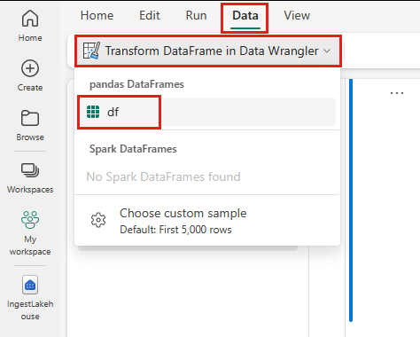
- Under the notebook ribbon Data tab, select Launch Data Wrangler. You'll see a list of activated pandas DataFrames available for editing.
- Select the DataFrame you wish to open in Data Wrangler. Since this notebook only contains one DataFrame,
df, selectdf.
Data Wrangler launches and generates a descriptive overview of your data. The table in the middle shows each data column. The Summary panel next to the table shows information about the DataFrame. When you select a column in the table, the summary updates with information about the selected column. In some instances, the data displayed and summarized will be a truncated view of your DataFrame. When this happens, you'll see warning image in the summary pane. Hover over this warning to view text explaining the situation.

Each operation you do can be applied in a matter of clicks, updating the data display in real time and generating code that you can save back to your notebook as a reusable function.
The rest of this section walks you through the steps to perform data cleaning with Data Wrangler.
Drop duplicate rows
On the left panel is a list of operations (such as Find and replace, Format, Formulas, Numeric) you can perform on the dataset.
Expand Find and replace and select Drop duplicate rows.
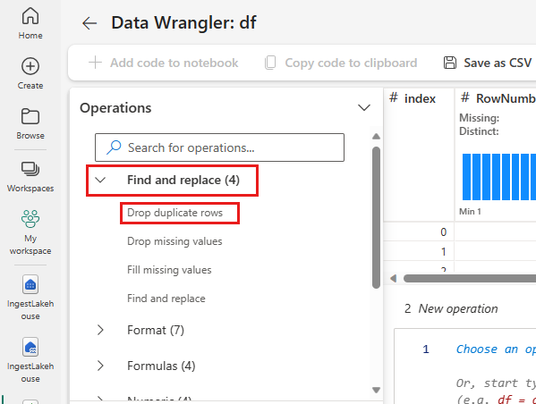
A panel appears for you to select the list of columns you want to compare to define a duplicate row. Select RowNumber and CustomerId.
In the middle panel is a preview of the results of this operation. Under the preview is the code to perform the operation. In this instance, the data appears to be unchanged. But since you're looking at a truncated view, it's a good idea to still apply the operation.
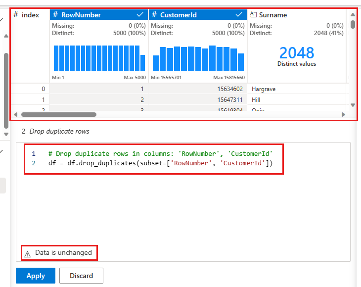
Select Apply (either at the side or at the bottom) to go to the next step.

Drop rows with missing data
Use Data Wrangler to drop rows with missing data across all columns.
Select Drop missing values from Find and replace.
Choose Select all from the Target columns.

Select Apply to go on to the next step.

Drop columns
Use Data Wrangler to drop columns that you don't need.
Expand Schema and select Drop columns.
Select RowNumber, CustomerId, Surname. These columns appear in red in the preview, to show they're changed by the code (in this case, dropped.)
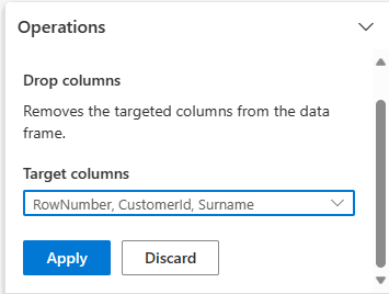
Select Apply to go on to the next step.

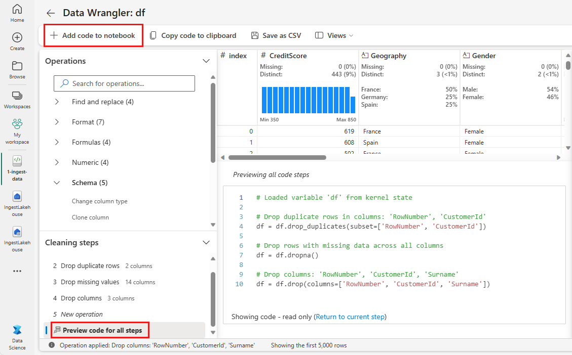
Add code to notebook
Each time you select Apply, a new step is created in the Cleaning steps panel on the bottom left. At the bottom of the panel, select Preview code for all steps to view a combination of all the separate steps.
Select Add code to notebook at the top left to close Data Wrangler and add the code automatically. The Add code to notebook wraps the code in a function, then calls the function.
Tip
The code generated by Data Wrangler won't be applied until you manually run the new cell.
If you didn't use Data Wrangler, you can instead use this next code cell.
This code is similar to the code produced by Data Wrangler, but adds in the argument inplace=True to each of the generated steps. By setting inplace=True, pandas will overwrite the original DataFrame instead of producing a new DataFrame as an output.
# Modified version of code generated by Data Wrangler
# Modification is to add in-place=True to each step

# Define a new function that include all above Data Wrangler operations
def clean_data(df):
    # Drop rows with missing data across all columns
    df.dropna(inplace=True)
    # Drop duplicate rows in columns: 'RowNumber', 'CustomerId'
    df.drop_duplicates(subset=['RowNumber', 'CustomerId'], inplace=True)
    # Drop columns: 'RowNumber', 'CustomerId', 'Surname'
    df.drop(columns=['RowNumber', 'CustomerId', 'Surname'], inplace=True)
    return df

df_clean = clean_data(df.copy())
df_clean.head()
Explore the data
Display some summaries and visualizations of the cleaned data.
Determine categorical, numerical, and target attributes
Use this code to determine categorical, numerical, and target attributes.
# Determine the dependent (target) attribute
dependent_variable_name = "Exited"
print(dependent_variable_name)
# Determine the categorical attributes
categorical_variables = [col for col in df_clean.columns if col in "O"
                        or df_clean[col].nunique() <=5
                        and col not in "Exited"]
print(categorical_variables)
# Determine the numerical attributes
numeric_variables = [col for col in df_clean.columns if df_clean[col].dtype != "object"
                        and df_clean[col].nunique() >5]
print(numeric_variables)
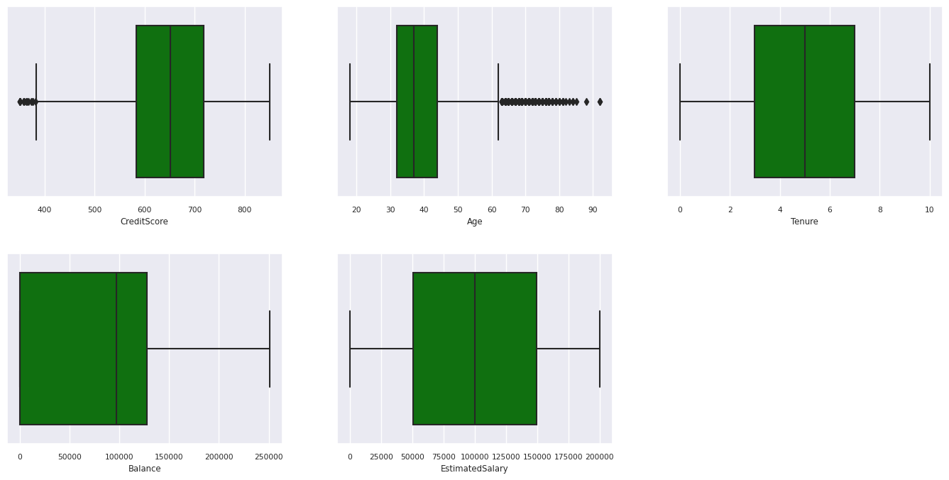
The five-number summary
Show the five-number summary (the minimum score, first quartile, median, third quartile, the maximum score) for the numerical attributes, using box plots.
df_num_cols = df_clean[numeric_variables]
sns.set(font_scale = 0.7)
fig, axes = plt.subplots(nrows = 2, ncols = 3, gridspec_kw =  dict(hspace=0.3), figsize = (17,8))
fig.tight_layout()
for ax,col in zip(axes.flatten(), df_num_cols.columns):
    sns.boxplot(x = df_num_cols[col], color='green', ax = ax)
fig.delaxes(axes[1,2])
Distribution of exited and nonexited customers
Show the distribution of exited versus nonexited customers across the categorical attributes.
df_clean['Exited'] = df_clean['Exited'].astype(str)
attr_list = ['Geography', 'Gender', 'HasCrCard', 'IsActiveMember', 'NumOfProducts', 'Tenure']
df_clean['Exited'] = df_clean['Exited'].astype(str)
fig, axarr = plt.subplots(2, 3, figsize=(15, 4))
for ind, item in enumerate (attr_list):
    print(ind, item)
    sns.countplot(x = item, hue = 'Exited', data = df_clean, ax = axarr[ind%2][ind//2])
fig.subplots_adjust(hspace=0.7)
df_clean['Exited'] = df_clean['Exited'].astype(int)

Distribution of numerical attributes
Show the frequency distribution of numerical attributes using histogram.
columns = df_num_cols.columns[: len(df_num_cols.columns)]
fig = plt.figure()
fig.set_size_inches(18, 8)
length = len(columns)
for i,j in itertools.zip_longest(columns, range(length)):
    plt.subplot((length // 2), 3, j+1)
    plt.subplots_adjust(wspace = 0.2, hspace = 0.5)
    df_num_cols[i].hist(bins = 20, edgecolor = 'black')
    plt.title(i)
plt.show()

Perform feature engineering
Perform feature engineering to generate new attributes based on current attributes:
df_clean['Tenure'] = df_clean['Tenure'].astype(int)
df_clean["NewTenure"] = df_clean["Tenure"]/df_clean["Age"]
df_clean["NewCreditsScore"] = pd.qcut(df_clean['CreditScore'], 6, labels = [1, 2, 3, 4, 5, 6])
df_clean["NewAgeScore"] = pd.qcut(df_clean['Age'], 8, labels = [1, 2, 3, 4, 5, 6, 7, 8])
df_clean["NewBalanceScore"] = pd.qcut(df_clean['Balance'].rank(method="first"), 5, labels = [1, 2, 3, 4, 5])
df_clean["NewEstSalaryScore"] = pd.qcut(df_clean['EstimatedSalary'], 10, labels = [1, 2, 3, 4, 5, 6, 7, 8, 9, 10])
Use Data Wrangler to perform one-hot encoding
Data Wrangler can also be used to perform one-hot encoding. To do so, re-open Data Wrangler. This time, select the df_clean data.
- Expand Formulas and select One-hot encode.
- A panel appears for you to select the list of columns you want to perform one-hot encoding on. Select Geography and Gender.
You could copy the generated code, close Data Wrangler to return to the notebook, then paste into a new cell. Or, select Add code to notebook at the top left to close Data Wrangler and add the code automatically.
If you didn't use Data Wrangler, you can instead use this next code cell:
# This is the same code that Data Wrangler will generate

import pandas as pd

def clean_data(df_clean):
    # One-hot encode columns: 'Geography', 'Gender'
    for column in ['Geography', 'Gender']:
        insert_loc = df_clean.columns.get_loc(column)
        df_clean = pd.concat([df_clean.iloc[:,:insert_loc], pd.get_dummies(df_clean.loc[:, [column]]), df_clean.iloc[:,insert_loc+1:]], axis=1)
    return df_clean

df_clean_1 = clean_data(df_clean.copy())
df_clean_1.head()
# This is the same code that Data Wrangler will generate

import pandas as pd

def clean_data(df_clean):
    # One-hot encode columns: 'Geography', 'Gender'
    df_clean = pd.get_dummies(df_clean, columns=['Geography', 'Gender'])
    return df_clean

df_clean_1 = clean_data(df_clean.copy())
df_clean_1.head()
Summary of observations from the exploratory data analysis
- Most of the customers are from France comparing to Spain and Germany, while Spain has the lowest churn rate comparing to France and Germany.
- Most of the customers have credit cards.
- There are customers whose age and credit score are above 60 and below 400, respectively, but they can't be considered as outliers.
- Very few customers have more than two of the bank's products.
- Customers who aren't active have a higher churn rate.
- Gender and tenure years don't seem to have an impact on customer's decision to close the bank account.
Create a delta table for the cleaned data
You'll use this data in the next notebook of this series.
table_name = "df_clean"
# Create Spark DataFrame from pandas
sparkDF=spark.createDataFrame(df_clean_1)
sparkDF.write.mode("overwrite").format("delta").save(f"Tables/{table_name}")
print(f"Spark dataframe saved to delta table: {table_name}")
Next step
Train and register machine learning models with this data: