Tutorial Part 3: Train and register a machine learning model

In this tutorial, you'll learn to train multiple machine learning models to select the best one in order to predict which bank customers are likely to leave.

In this tutorial, you'll:

• Train Random Forrest and LightGBM models.
• Use Microsoft Fabric's native integration with the MLflow framework to log the trained machine learning models, the used hyperaparameters, and evaluation metrics.
• Register the trained machine learning model.
• Assess the performances of the trained machine learning models on the validation dataset.

MLflow is an open source platform for managing the machine learning lifecycle with features like Tracking, Models, and Model Registry. MLflow is natively integrated with the Fabric Data Science experience.

Prerequisites

• Get a Microsoft Fabric subscription. Or, sign up for a free Microsoft Fabric trial.

• Sign in to Microsoft Fabric.

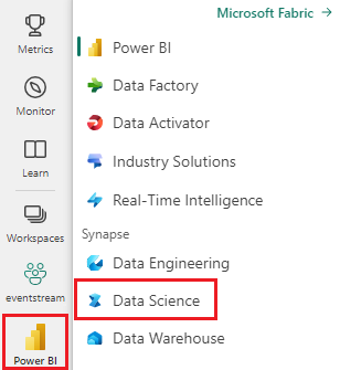
• Use the experience switcher on the left side of your home page to switch to the Synapse Data Science experience.

  

This is part 3 of 5 in the tutorial series. To complete this tutorial, first complete:

• Part 1: Ingest data into a Microsoft Fabric lakehouse using Apache Spark.
• Part 2: Explore and visualize data using Microsoft Fabric notebooks to learn more about the data.

Follow along in notebook

3-train-evaluate.ipynb is the notebook that accompanies this tutorial.

To open the accompanying notebook for this tutorial, follow the instructions in Prepare your system for data science tutorials, to import the notebook to your workspace.

If you'd rather copy and paste the code from this page, you can create a new notebook.

Be sure to attach a lakehouse to the notebook before you start running code.

Important

Attach the same lakehouse you used in part 1 and part 2.

Install custom libraries

For this notebook, you'll install imbalanced-learn (imported as imblearn) using %pip install. Imbalanced-learn is a library for Synthetic Minority Oversampling Technique (SMOTE) which is used when dealing with imbalanced datasets. The PySpark kernel will be restarted after %pip install, so you'll need to install the library before you run any other cells.

You'll access SMOTE using the imblearn library. Install it now using the in-line installation capabilities (e.g., %pip, %conda).

# Install imblearn for SMOTE using pip
%pip install imblearn

Important

Run this install each time you restart the notebook.

When you install a library in a notebook, it's only available for the duration of the notebook session and not in the workspace. If you restart the notebook, you'll need to install the library again.

If you have a library you often use, and you want to make it available to all notebooks in your workspace, you can use a Fabric environment for that purpose. You can create an environment, install the library in it, and then your workspace admin can attach the environment to the workspace as its default environment. For more information on setting an environment as the workspace default, see Admin sets default libraries for the workspace.

For information on migrating existing workspace libraries and Spark properties to an environment, see Migrate workspace libraries and Spark properties to a default environment.

Load the data

Prior to training any machine learning model, you need to load the delta table from the lakehouse in order to read the cleaned data you created in the previous notebook.

import pandas as pd
SEED = 12345
df_clean = spark.read.format("delta").load("Tables/df_clean").toPandas()

Generate experiment for tracking and logging the model using MLflow

This section demonstrates how to generate an experiment, specify the machine learning model and training parameters as well as scoring metrics, train the machine learning models, log them, and save the trained models for later use.

import mlflow
# Setup experiment name
EXPERIMENT_NAME = "bank-churn-experiment"  # MLflow experiment name

Extending the MLflow autologging capabilities, autologging works by automatically capturing the values of input parameters and output metrics of a machine learning model as it is being trained. This information is then logged to your workspace, where it can be accessed and visualized using the MLflow APIs or the corresponding experiment in your workspace.

All the experiments with their respective names are logged and you'll be able to track their parameters and performance metrics. To learn more about autologging, see Autologging in Microsoft Fabric.

Set experiment and autologging specifications

mlflow.set_experiment(EXPERIMENT_NAME)
mlflow.autolog(exclusive=False)

Import scikit-learn and LightGBM

With your data in place, you can now define the machine learning models. You'll apply Random Forrest and LightGBM models in this notebook. Use scikit-learn and lightgbm to implement the models within a few lines of code.

# Import the required libraries for model training
from sklearn.model_selection import train_test_split
from lightgbm import LGBMClassifier
from sklearn.ensemble import RandomForestClassifier
from sklearn.metrics import accuracy_score, f1_score, precision_score, confusion_matrix, recall_score, roc_auc_score, classification_report

Prepare training, validation and test datasets

Use the train_test_split function from scikit-learn to split the data into training, validation, and test sets.

y = df_clean["Exited"]
X = df_clean.drop("Exited",axis=1)
# Split the dataset to 60%, 20%, 20% for training, validation, and test datasets
# Train-Test Separation
X_train, X_test, y_train, y_test = train_test_split(X, y, test_size=0.20, random_state=SEED)
# Train-Validation Separation
X_train, X_val, y_train, y_val = train_test_split(X_train, y_train, test_size=0.25, random_state=SEED)

Save test data to a delta table

Save the test data to the delta table for use in the next notebook.

table_name = "df_test"
# Create PySpark DataFrame from Pandas
df_test=spark.createDataFrame(X_test)
df_test.write.mode("overwrite").format("delta").save(f"Tables/{table_name}")
print(f"Spark test DataFrame saved to delta table: {table_name}")

Apply SMOTE to the training data to synthesize new samples for the minority class

The data exploration in part 2 showed that out of the 10,000 data points corresponding to 10,000 customers, only 2,037 customers (around 20%) have left the bank. This indicates that the dataset is highly imbalanced. The problem with imbalanced classification is that there are too few examples of the minority class for a model to effectively learn the decision boundary. SMOTE is the most widely used approach to synthesize new samples for the minority class. Learn more about SMOTE here and here.

Tip

Note that SMOTE should only be applied to the training dataset. You must leave the test dataset in its original imbalanced distribution in order to get a valid approximation of how the machine learning model will perform on the original data, which is representing the situation in production.

from collections import Counter
from imblearn.over_sampling import SMOTE

sm = SMOTE(random_state=SEED)
X_res, y_res = sm.fit_resample(X_train, y_train)
new_train = pd.concat([X_res, y_res], axis=1)

Tip

You can safely ignore the MLflow warning message that appears when you run this cell. If you see a ModuleNotFoundError message, you missed running the first cell in this notebook, which installs the imblearn library. You need to install this library each time you restart the notebook. Go back and re-run all the cells starting with the first cell in this notebook.

Model training

• Train the model using Random Forest with maximum depth of 4 and 4 features

mlflow.sklearn.autolog(registered_model_name='rfc1_sm') # Register the trained model with autologging
rfc1_sm = RandomForestClassifier(max_depth=4, max_features=4, min_samples_split=3, random_state=1) # Pass hyperparameters
with mlflow.start_run(run_name="rfc1_sm") as run:
    rfc1_sm_run_id = run.info.run_id # Capture run_id for model prediction later
    print("run_id: {}; status: {}".format(rfc1_sm_run_id, run.info.status))
    # rfc1.fit(X_train,y_train) # Imbalanaced training data
    rfc1_sm.fit(X_res, y_res.ravel()) # Balanced training data
    rfc1_sm.score(X_val, y_val)
    y_pred = rfc1_sm.predict(X_val)
    cr_rfc1_sm = classification_report(y_val, y_pred)
    cm_rfc1_sm = confusion_matrix(y_val, y_pred)
    roc_auc_rfc1_sm = roc_auc_score(y_res, rfc1_sm.predict_proba(X_res)[:, 1])

• Train the model using Random Forest with maximum depth of 8 and 6 features

mlflow.sklearn.autolog(registered_model_name='rfc2_sm') # Register the trained model with autologging
rfc2_sm = RandomForestClassifier(max_depth=8, max_features=6, min_samples_split=3, random_state=1) # Pass hyperparameters
with mlflow.start_run(run_name="rfc2_sm") as run:
    rfc2_sm_run_id = run.info.run_id # Capture run_id for model prediction later
    print("run_id: {}; status: {}".format(rfc2_sm_run_id, run.info.status))
    # rfc2.fit(X_train,y_train) # Imbalanced training data
    rfc2_sm.fit(X_res, y_res.ravel()) # Balanced training data
    rfc2_sm.score(X_val, y_val)
    y_pred = rfc2_sm.predict(X_val)
    cr_rfc2_sm = classification_report(y_val, y_pred)
    cm_rfc2_sm = confusion_matrix(y_val, y_pred)
    roc_auc_rfc2_sm = roc_auc_score(y_res, rfc2_sm.predict_proba(X_res)[:, 1])

• Train the model using LightGBM

# lgbm_model
mlflow.lightgbm.autolog(registered_model_name='lgbm_sm') # Register the trained model with autologging
lgbm_sm_model = LGBMClassifier(learning_rate = 0.07, 
                        max_delta_step = 2, 
                        n_estimators = 100,
                        max_depth = 10, 
                        eval_metric = "logloss", 
                        objective='binary', 
                        random_state=42)

with mlflow.start_run(run_name="lgbm_sm") as run:
    lgbm1_sm_run_id = run.info.run_id # Capture run_id for model prediction later
    # lgbm_sm_model.fit(X_train,y_train) # Imbalanced training data
    lgbm_sm_model.fit(X_res, y_res.ravel()) # Balanced training data
    y_pred = lgbm_sm_model.predict(X_val)
    accuracy = accuracy_score(y_val, y_pred)
    cr_lgbm_sm = classification_report(y_val, y_pred)
    cm_lgbm_sm = confusion_matrix(y_val, y_pred)
    roc_auc_lgbm_sm = roc_auc_score(y_res, lgbm_sm_model.predict_proba(X_res)[:, 1])

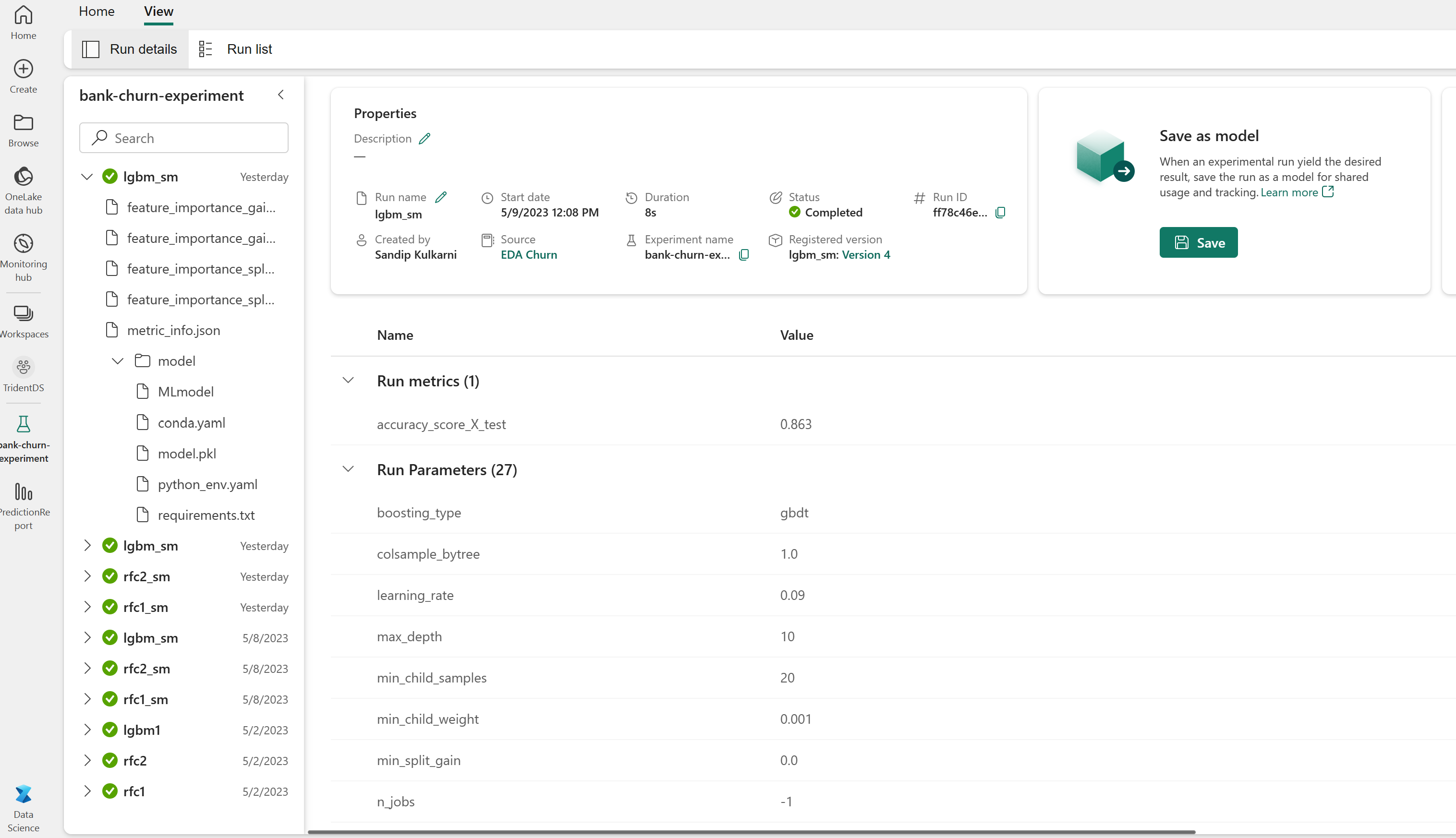
Experiments artifact for tracking model performance

The experiment runs are automatically saved in the experiment artifact that can be found from the workspace. They're named based on the name used for setting the experiment. All of the trained machine learning models, their runs, performance metrics, and model parameters are logged.

To view your experiments:

1. On the left panel, select your workspace.

2. On the top right, filter to show only experiments, to make it easier to find the experiment you're looking for.

   

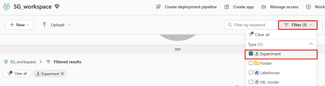
3. Find and select the experiment name, in this case bank-churn-experiment. If you don't see the experiment in your workspace, refresh your browser.

   

Assess the performances of the trained models on the validation dataset

Once done with machine learning model training, you can assess the performance of trained models in two ways.

• Open the saved experiment from the workspace, load the machine learning models, and then assess the performance of the loaded models on the validation dataset.

  # Define run_uri to fetch the model
  # mlflow client: mlflow.model.url, list model
  load_model_rfc1_sm = mlflow.sklearn.load_model(f"runs:/{rfc1_sm_run_id}/model")
  load_model_rfc2_sm = mlflow.sklearn.load_model(f"runs:/{rfc2_sm_run_id}/model")
  load_model_lgbm1_sm = mlflow.lightgbm.load_model(f"runs:/{lgbm1_sm_run_id}/model")
  # Assess the performance of the loaded model on validation dataset
  ypred_rfc1_sm_v1 = load_model_rfc1_sm.predict(X_val) # Random Forest with max depth of 4 and 4 features
  ypred_rfc2_sm_v1 = load_model_rfc2_sm.predict(X_val) # Random Forest with max depth of 8 and 6 features
  ypred_lgbm1_sm_v1 = load_model_lgbm1_sm.predict(X_val) # LightGBM
  

• Directly assess the performance of the trained machine learning models on the validation dataset.

  ypred_rfc1_sm_v2 = rfc1_sm.predict(X_val) # Random Forest with max depth of 4 and 4 features
  ypred_rfc2_sm_v2 = rfc2_sm.predict(X_val) # Random Forest with max depth of 8 and 6 features
  ypred_lgbm1_sm_v2 = lgbm_sm_model.predict(X_val) # LightGBM
  

Depending on your preference, either approach is fine and should offer identical performances. In this notebook, you'll choose the first approach in order to better demonstrate the MLflow autologging capabilities in Microsoft Fabric.

Show True/False Positives/Negatives using the Confusion Matrix

Next, you'll develop a script to plot the confusion matrix in order to evaluate the accuracy of the classification using the validation dataset. The confusion matrix can be plotted using SynapseML tools as well, which is shown in Fraud Detection sample that is available here.

import seaborn as sns
sns.set_theme(style="whitegrid", palette="tab10", rc = {'figure.figsize':(9,6)})
import matplotlib.pyplot as plt
import matplotlib.ticker as mticker
from matplotlib import rc, rcParams
import numpy as np
import itertools

def plot_confusion_matrix(cm, classes,
                          normalize=False,
                          title='Confusion matrix',
                          cmap=plt.cm.Blues):
    print(cm)
    plt.figure(figsize=(4,4))
    plt.rcParams.update({'font.size': 10})
    plt.imshow(cm, interpolation='nearest', cmap=cmap)
    plt.title(title)
    plt.colorbar()
    tick_marks = np.arange(len(classes))
    plt.xticks(tick_marks, classes, rotation=45, color="blue")
    plt.yticks(tick_marks, classes, color="blue")

    fmt = '.2f' if normalize else 'd'
    thresh = cm.max() / 2.
    for i, j in itertools.product(range(cm.shape[0]), range(cm.shape[1])):
        plt.text(j, i, format(cm[i, j], fmt),
                 horizontalalignment="center",
                 color="red" if cm[i, j] > thresh else "black")

    plt.tight_layout()
    plt.ylabel('True label')
    plt.xlabel('Predicted label')

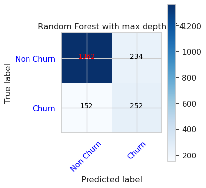
• Confusion Matrix for Random Forest Classifier with maximum depth of 4 and 4 features

cfm = confusion_matrix(y_val, y_pred=ypred_rfc1_sm_v1)
plot_confusion_matrix(cfm, classes=['Non Churn','Churn'],
                      title='Random Forest with max depth of 4')
tn, fp, fn, tp = cfm.ravel()

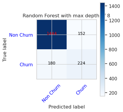
• Confusion Matrix for Random Forest Classifier with maximum depth of 8 and 6 features

cfm = confusion_matrix(y_val, y_pred=ypred_rfc2_sm_v1)
plot_confusion_matrix(cfm, classes=['Non Churn','Churn'],
                      title='Random Forest with max depth of 8')
tn, fp, fn, tp = cfm.ravel()

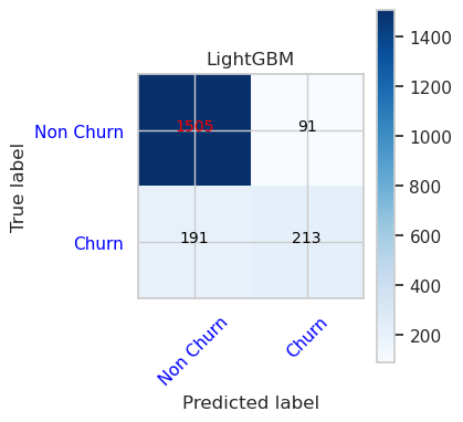
• Confusion Matrix for LightGBM

cfm = confusion_matrix(y_val, y_pred=ypred_lgbm1_sm_v1)
plot_confusion_matrix(cfm, classes=['Non Churn','Churn'],
                      title='LightGBM')
tn, fp, fn, tp = cfm.ravel()

Next step

Part 4: Perform batch scoring and save predictions to a lakehouse