Quickstart: Create your first dataflow to get and transform data
Dataflows are a self-service, cloud-based, data preparation technology. In this article, you create your first dataflow, get data for your dataflow, then transform the data and publish the dataflow.
Prerequisites
The following prerequisites are required before you start:
- A Microsoft Fabric tenant account with an active subscription. Create a free account.
- Make sure you have a Microsoft Fabric enabled Workspace: Create a workspace.
Create a dataflow
In this section, you're creating your first dataflow.
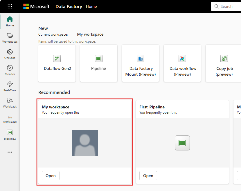
Switch to the Data factory experience.
Navigate to your Microsoft Fabric workspace.
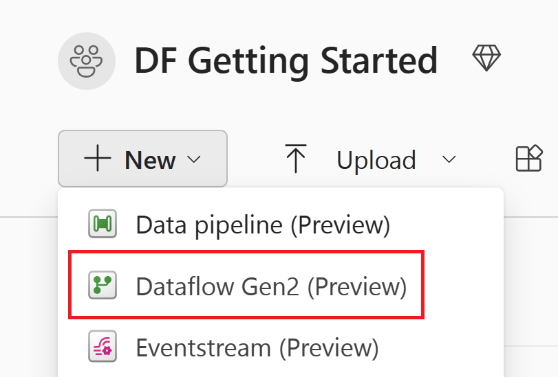
Select New, and then select Dataflow Gen2.

Get data
Let's get some data! In this example, you're getting data from an OData service. Use the following steps to get data in your dataflow.
In the dataflow editor, select Get data and then select More.

In Choose data source, select View more.
In New source, select Other > OData as the data source.
Enter the URL
https://services.odata.org/v4/northwind/northwind.svc/, and then select Next.
Select the Orders and Customers tables, and then select Create.
You can learn more about the get data experience and functionality at Getting data overview.
Apply transformations and publish
You loaded your data into your first dataflow now. Congratulations! Now it's time to apply a couple of transformations in order to bring this data into the desired shape.
You do this task from the Power Query editor. You can find a detailed overview of the Power Query editor at The Power Query user interface.
Follow these steps to apply transformations and publish:
Ensure that the Data Profiling tools are enabled by navigating to Home > Options > Global Options.

Also make sure you enable the diagram view using the options under the View tab in the Power Query editor ribbon, or by selecting the diagram view icon on the lower right side of the Power Query window.
Within the Orders table, you calculate the total number of orders per customer. To achieve this goal, select the CustomerID column in the data preview and then select Group By under the Transform tab in the ribbon.
You perform a count of rows as the aggregation within Group By. You can learn more about Group By capabilities at Grouping or summarizing rows.

After grouping data in the Orders table, we'll obtain a two-column table with CustomerID and Count as the columns.
Next, you want to combine data from the Customers table with the Count of Orders per customer. To combine data, select the Customers query in the Diagram View and use the "⋮" menu to access the Merge queries as new transformation.
Configure the Merge operation as shown in the following screenshot by selecting CustomerID as the matching column in both tables. Then select Ok.

Screenshot of the Merge window, with the Left table for merge set to the Customers table and the Right table for merge set to the Orders table. The CustomerID column is selected for both the Customers and Orders tables. Also, the Join Kind is set to Left outer. All other selections are set to their default value.
Upon performing the Merge queries as new operation, you obtain a new query with all columns from the Customers table and one column with nested data from the Orders table.
In this example, you're only interested in a subset of columns in the Customers table. You select those columns by using the schema view. Enable the schema view within the toggle button on the bottom-right corner of the dataflows editor.
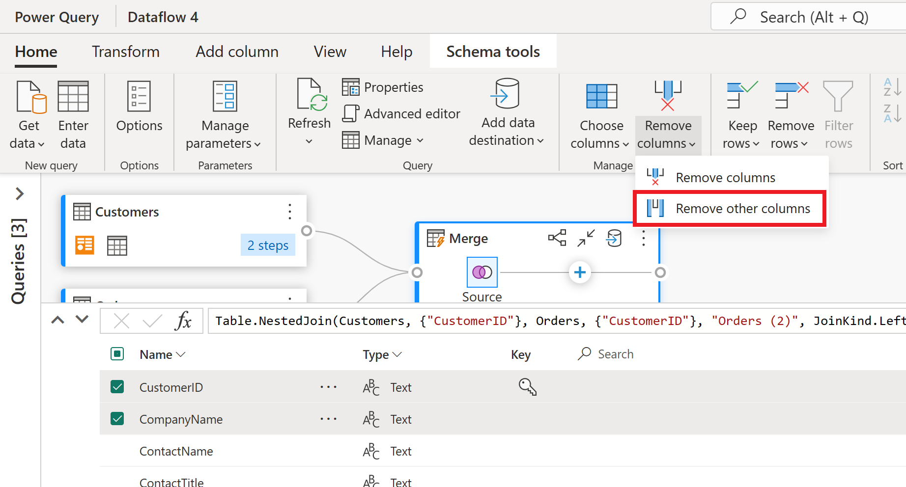
The schema view provides a focused view into a table’s schema information, including column names and data types. Schema view has a set of schema tools available through a contextual ribbon tab. In this scenario, you select the CustomerID, CompanyName, and Orders (2) columns, then select the Remove columns button, and then select Remove other columns in the Schema tools tab.

The Orders (2) column contains nested information resulting from the merge operation you performed a few steps ago. Now, switch back to the data view by selecting the Show data view button next to the Show schema view button in the bottom-right corner of the UI. Then use the Expand Column transformation in the Orders (2) column header to select the Count column.
As the final operation, you want to rank your customers based on their number of orders. Select the Count column and then select the Rank column button under the Add Column tab in the ribbon.
Keep the default settings in Rank Column. Then select OK to apply this transformation.

Now rename the resulting query as Ranked Customers using the Query settings pane on the right side of the screen.
Now that you finished transforming and combining your data, you can configure its output destination settings. Select Choose data destination at the bottom of the Query settings pane.
For this step, you can configure an output to your lakehouse if you have one available, or skip this step if you don't. Within this experience, you're able to configure the destination lakehouse and table for your query results, in addition to the update method (Append or Replace).
Your dataflow is now ready to be published. Review the queries in the diagram view, and then select Publish.
You're now returned to the workspace. A spinner icon next to your dataflow name indicates publishing is in progress. Once the publishing completes, your dataflow is ready to refresh!
Important
When the first Dataflow Gen2 is created in a workspace, Lakehouse and Warehouse items are provisioned along with their related SQL analytics endpoint and semantic models. These items are shared by all dataflows in the workspace and are required for Dataflow Gen2 to operate, shouldn't be deleted, and aren't intended to be used directly by users. The items are an implementation detail of Dataflow Gen2. The items aren't visible in the workspace, but might be accessible in other experiences such as the Notebook, SQL analytics endpoint, Lakehouse, and Warehouse experiences. You can recognize the items by their prefix in the name. The prefix of the items is `DataflowsStaging'.
In your workspace, select the Schedule Refresh icon.

Turn on the scheduled refresh, select Add another time, and configure the refresh as shown in the following screenshot.

Screenshot of the scheduled refresh options, with scheduled refresh turned on, the refresh frequency set to Daily, the Time zone set to coordinated universal time, and the Time set to 4:00 AM. The on button, the Add another time selection, the dataflow owner, and the apply button are all emphasized.
Clean up resources
If you're not going to continue to use this dataflow, delete the dataflow using the following steps:
Navigate to your Microsoft Fabric workspace.

Select the vertical ellipsis next to the name of your dataflow and then select Delete.

Select Delete to confirm the deletion of your dataflow.

Related content
The dataflow in this sample shows you how to load and transform data in Dataflow Gen2. You learned how to:
- Create a Dataflow Gen2.
- Transform data.
- Configure destination settings for transformed data.
- Run and schedule your data pipeline.
Advance to the next article to learn how to create your first data pipeline.


