SKI と CLI で時系列予測モデルをトレーニングするために、AutoML を設定する
適用対象: Azure CLI ml extension v2 (現行)Python SDK azure-ai-ml v2 (現行)
この記事では、Azure Machine Learning Python SDK で、Azure Machine Learning 自動 ML を使用した時系列予測のために、AutoML を設定する方法を説明します。
これを行うには、次の手順を実行します。
- トレーニング用のデータを準備します。
- 予測ジョブで特定の時系列パラメーターを構成します。
- コンポーネントとパイプラインを使用してトレーニング、推論、モデル評価をオーケストレーションします。
Azure Machine Learning スタジオの自動 ML を使用して、ロー コードで時系列予測を行う例は、「チュートリアル:自動機械学習を使用して需要を予測する」をご覧ください。
AutoML では、標準の機械学習モデルと既知の時系列モデルを使用して予測を作成します。 このアプローチでは、ターゲット変数に関する履歴情報、入力データ内のユーザー指定の機能、および自動的に設計された機能が組み込まれています。 そして、モデル検索アルゴリズムが最適な予測精度のモデルを見つけるために動作します。 詳細については、予測手法とモデル検索に関する記事を参照してください。
前提条件
この記事では、以下が必要です。
Azure Machine Learning ワークスペース。 ワークスペースを作成するには、「ワークスペース リソースの作成」を参照してください。
AutoML トレーニング ジョブを起動できること。 詳細については、AutoML の設定に関する攻略ガイドに従ってください。
データをトレーニングして検証する
AutoML 予測の入力データには、有効な時系列が表形式で含まれている必要があります。 各変数には、それに対応する独自の列がデータ テーブルに入っている必要があります。 AutoML には、少なくとも 2 つの列 (時間軸を表す時間列と、予測する数量であるターゲット列) が必要です。 他の列は予測器として機能します。 詳細については、「AutoML でのデータの使用方法」を参照してください。
重要
将来の値を予測するためにモデルをトレーニングするときは、目的のトレーニングで使用されるすべての機能が、意図した期間の予測を実行するときに使用できることを確認してください。
たとえば、現在の株価の特徴を含めれば、トレーニングの精度を大幅に高めることができます。 ただし、長期間にわたり予測する予定の場合、将来の時系列ポイントに応じた将来の株価を正確に予測できない可能性があり、モデルの精度が低下することがあります。
AutoML 予測ジョブでは、トレーニング データが MLTable オブジェクトとして表される必要があります。 MLTable では、データ ソースと、データを読み込む手順を指定します。 詳細とユース ケースについては、MLTable の攻略ガイドを参照してください。 簡単な例として、トレーニング データがローカル ディレクトリ ./train_data/timeseries_train.csv の CSV ファイルに含まれているとします。
次の例に示すように、mltable Python SDK を使用して MLTable を作成できます。
import mltable

paths = [
    {'file': './train_data/timeseries_train.csv'}
]

train_table = mltable.from_delimited_files(paths)
train_table.save('./train_data')
このコードは、ファイル形式と読み込み手順が含間れた新しいファイル ./train_data/MLTable を作成します。
次に、以下のように、Azure Machine Learning Python SDK を使用して、トレーニング ジョブを開始するために必要な入力データ オブジェクトを定義します。
from azure.ai.ml.constants import AssetTypes
from azure.ai.ml import Input

# Training MLTable defined locally, with local data to be uploaded
my_training_data_input = Input(
    type=AssetTypes.MLTABLE, path="./train_data"
)
検証データの指定も同様に行います。MLTable を作成し、検証データ入力を指定します。 または、検証データを指定しない場合、AutoML によってトレーニング データからクロス検証分割が自動的に作成され、モデルの選択に使用されます。 詳細については、予測モデルの選択に関する記事を参照してください。 予測モデルを正常にトレーニングするために必要なトレーニング データの量の詳細については、トレーニング データの長さの要件に関する記事も参照してください。
AutoML でクロス検証を適用してオーバーフィットを防止する方法について、詳細情報をご覧ください。
実験を実行するために計算する
AutoML では、フル マネージド コンピューティング リソースである Azure Machine Learning コンピューティングを使用してトレーニング ジョブを実行します。 次の例では、cpu-compute という名前のコンピューティング クラスターが作成されます。
from azure.ai.ml.entities import AmlCompute

# specify aml compute name.
cpu_compute_target = "cpu-cluster"

try:
    ml_client.compute.get(cpu_compute_target)
except Exception:
    print("Creating a new cpu compute target...")
    compute = AmlCompute(
        name=cpu_compute_target, size="STANDARD_D2_V2", min_instances=0, max_instances=4
    )
ml_client.compute.begin_create_or_update(compute).result()実験を構成する
automl ファクトリ関数を使用して、Python SDK で予測ジョブを構成します。 次の例は、プライマリ メトリックを設定して予測ジョブを作成し、トレーニング実行で制限を設定する方法を示しています。
from azure.ai.ml import automl

# note that the below is a code snippet -- you might have to modify the variable values to run it successfully
forecasting_job = automl.forecasting(
    compute="cpu-compute",
    experiment_name="sdk-v2-automl-forecasting-job",
    training_data=my_training_data_input,
    target_column_name=target_column_name,
    primary_metric="normalized_root_mean_squared_error",
    n_cross_validations="auto",
)

# Limits are all optional
forecasting_job.set_limits(
    timeout_minutes=120,
    trial_timeout_minutes=30,
    max_concurrent_trials=4,
)
予測ジョブの設定
予測タスクには、予測固有の多くの設定があります。 これらの設定の最も基本的なものは、トレーニング データの時間列の名前と予測期間です。
ForecastingJob メソッドを使用して、次の設定を構成します。
# Forecasting specific configuration
forecasting_job.set_forecast_settings(
    time_column_name=time_column_name,
    forecast_horizon=24
)
時間列の名前は必須の設定であり、予測許可は通常、予測シナリオに従って設定する必要があります。 データに複数の時系列が含まれている場合は、時系列 ID 列の名前を指定できます。 これらの列をグループ化して、個々の系列を定義します。 たとえば、異なる店舗やブランドからの時間ごとの売上で構成されるデータがあるとします。 次の例では、データに "store" と "brand" という名前の列が含まれていると想定した場合の、時系列 ID 列の設定方法を示しています。
# Forecasting specific configuration
# Add time series IDs for store and brand
forecasting_job.set_forecast_settings(
    ...,  # other settings
    time_series_id_column_names=['store', 'brand']
)
AutoML では、何も指定されない場合、データ内の時系列 ID 列を自動的に検出しようとします。
その他の設定はオプションであり、次のセクションで確認します。
予測ジョブのオプション設定
ディープ ラーニングの有効化やターゲットのローリング ウィンドウ集計の指定など、予測タスクに対してオプションの構成を使用できます。 パラメーターの完全な一覧については、予測のリファレンス ドキュメントのドキュメントを参照してください。
モデルの検索設定
AutoML で最適なモデル allowed_training_algorithms と blocked_training_algorithms を検索するモデル空間を制御するオプション設定は、2 つあります。 探索空間を特定のモデル クラスのセットに制限するには、次の例のように allowed_training_algorithms パラメーターを使用します。
# Only search ExponentialSmoothing and ElasticNet models
forecasting_job.set_training(
    allowed_training_algorithms=["ExponentialSmoothing", "ElasticNet"]
)
この場合、予測ジョブでは、指数平滑法および Elastic Net モデル クラス "のみ" を検索します。 検索空間から特定のモデル クラス セットを削除するには、次の例のように blocked_training_algorithms を使用します。
# Search over all model classes except Prophet
forecasting_job.set_training(
    blocked_training_algorithms=["Prophet"]
)
これで、Prophet を "除く" すべてのモデル クラスがこのジョブで検索されます。 allowed_training_algorithms および blocked_training_algorithms で受け入れられる予測モデル名の一覧については、トレーニング プロパティのリファレンス ドキュメントを参照してください。 allowed_training_algorithms と blocked_training_algorithms の、両方ではなくいずれか一方を、トレーニング実行に適用できます。
ディープ ラーニングを有効にする
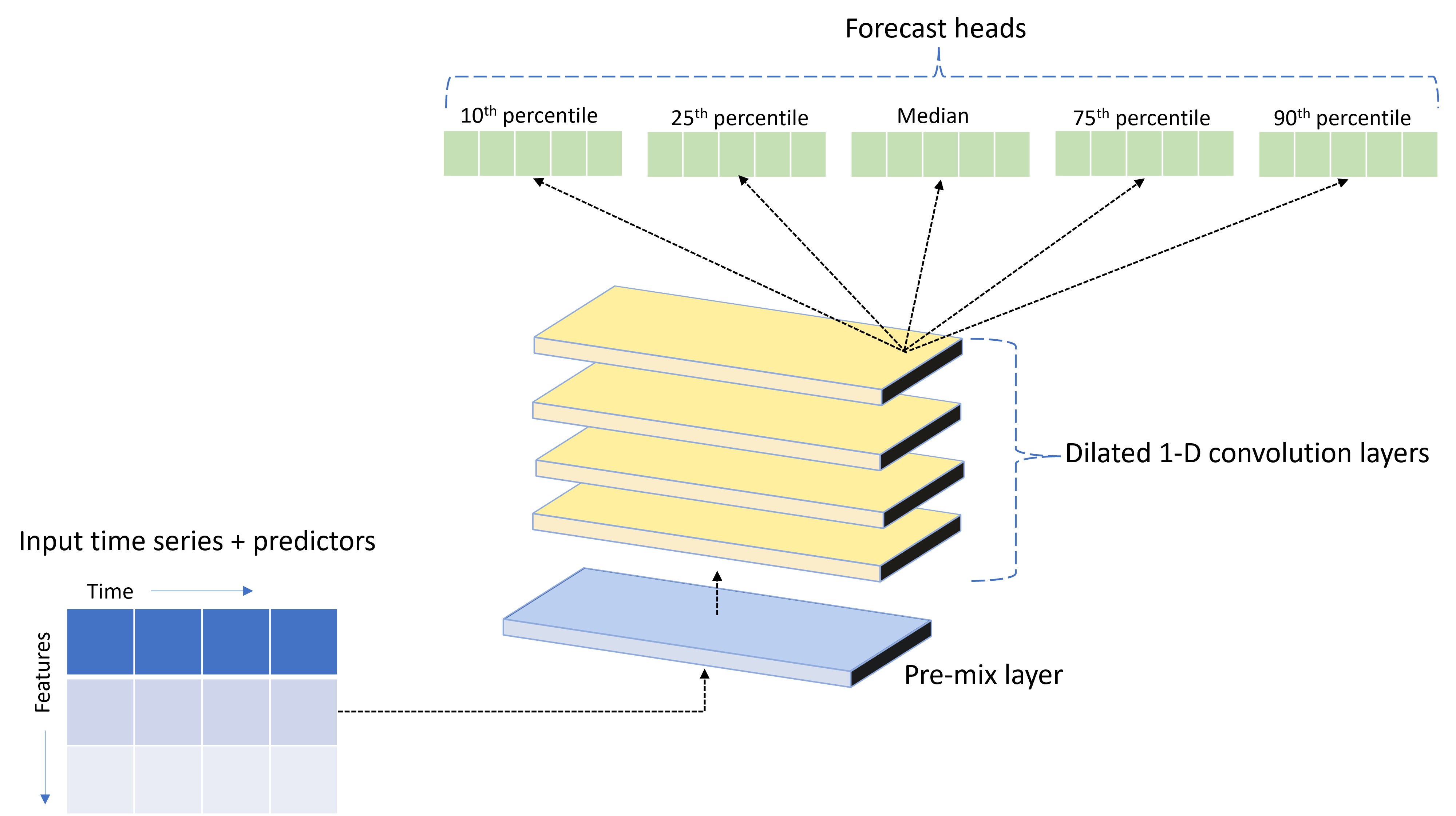
AutoML には、TCNForecaster と呼ばれるカスタムのディープ ニューラル ネットワーク (DNN) モデルが付属しています。 このモデルは、時系列モデリングに一般的なイメージング タスク メソッドを適用する、テンポラル畳み込みネットワーク (TCN) です。 つまり、1 次元 "因果" 畳み込みによってこのネットワークのバックボーンが形成され、モデルがトレーニング履歴の長期間にわたる複雑なパターンを学習できます。 詳細については、TCNForecaster の記事を参照してください。
TCNForecaster では、多くの場合、トレーニング履歴内に数千以上にもなる観測値があるときは標準の時系列モデルより高い精度を実現します。 ただし、それと同時に、容量が大きいため、TCNForecaster モデルのトレーニングとスイープに時間がかかります。
AutoML で TCNForecaster を有効にするには、次のようにトレーニング構成で enable_dnn_training フラグを設定します。
# Include TCNForecaster models in the model search
forecasting_job.set_training(
    enable_dnn_training=True
)
既定では、TCNForecaster トレーニングは、モデル試行ごとに、1 つのコンピューティング ノードと 1 つの GPU (使用可能な場合) に制限されます。 より大規模なデータ シナリオでは、複数のコア/GPU とノードに対して各 TCNForecaster 試行を分散させることをお勧めします。 詳細情報とコード サンプルについては、分散トレーニングに関する記事セクションを参照してください。
Azure Machine Learning スタジオで作成された AutoML 実験用の DNN を有効にするには、Studio UI 入門にあるタスクの種類の設定に関するページを参照してください。
注意
- SDK を使用して作成された実験に対して DNN を有効にすると、最適なモデル説明が無効になります。
- 自動機械学習での予測のための DNN サポートは、Databricks で開始して実行することはできません。
- DNN トレーニングが有効になっている場合、コンピューティングの種類には GPU をお勧めします
ラグとローリング ウィンドウの機能
ターゲットの最近の値は、多くの場合、予測モデルで影響力の大きい特徴です。 したがって、AutoML では、タイム ラグとローリング ウィンドウの集計機能を作成して、モデルの精度を向上させることができる可能性があります。
気象データと過去の需要が利用可能になっている、エネルギー需要予測のシナリオについて考えてみます。 この表は、ウィンドウ集計が直近 3 時間に適用されたときに発生する特徴エンジニアリングを示しています。 最小値、最大値、合計値の列は、定義された設定に基づいて、3 時間のスライディング ウィンドウで生成されます。 たとえば、2017 年 9 月 8 日の午前 4:00 に有効な観測値では、最大値、最小値、合計値は、2017 年 9 月 8 日午前 1:00 から午前 3:00 までの需要値を使用して計算されます。 この 3 時間のウィンドウは、残りの行のデータを設定するためにシフトされます。 詳細と例については、ラグ機能に関する記事を参照してください。

ローリング ウィンドウ サイズ (前の例では 3) と、作成したいラグ オーダーを設定することで、ターゲットのラグとローリング ウィンドウの集計機能を有効にすることができます。 feature_lags 設定を使用して、機能のラグを有効にすることもできます。 次の例では、これらの設定をすべて auto に設定して、AutoML がデータの相関構造を分析して設定を自動的に決定するようにします。
forecasting_job.set_forecast_settings(
    ...,  # other settings
    target_lags='auto',
    target_rolling_window_size='auto',
    feature_lags='auto'
)
短い系列の処理
自動 ML では、モデル開発のトレーニングと検証のフェーズを実施するのに十分なデータ ポイントがない場合、時系列は短い系列と見なされます。 長さの要件の詳細については、トレーニング データの長さの要件に関するページを参照してください。
AutoML には、短い系列に対して実行できるアクションがいくつか存在します。 これらのアクションは、short_series_handling_config 設定を使用して構成できます。 既定値は "auto" です。次の表では、設定について説明します。
| 設定 | 説明 |
|---|---|
auto |
短い系列処理の既定値。 - "すべての系列が短い" 場合は、データを埋め込みます。 - "すべてが短い系列というわけではない" 場合は、短い系列をドロップします。 |
pad |
short_series_handling_config = pad の場合、自動 ML によって、検出されたそれぞれの短い系列に対してランダムの値が追加されます。 次に、列の型と、それらに埋め込まれる内容を示します。- オブジェクト列には NAN - 数値列には 0 - ブール/論理列には False - ターゲット列にはホワイト ノイズが埋め込まれます。 |
drop |
short_series_handling_config = drop の場合、短い系列は自動 ML によってドロップされ、トレーニングや予測には使用されません。 これらの系列の予測では、NAN が返されます。 |
None |
埋め込まれる、またはドロップされる系列はありません。 |
次の例では、すべての短い系列が最小長にまで埋め込まれるように、短い系列の処理を設定します。
forecasting_job.set_forecast_settings(
    ...,  # other settings
    short_series_handling_config='pad'
)
警告
トレーニングの失敗を回避するために人為的なデータを用いているため、データの埋め込みは、結果のモデルの精度に影響する可能性があります。 短い系列が多くなる場合、説明可能性の結果に影響が生じる可能性があります。
頻度とターゲット データの集計
頻度とデータ集計のオプションを使用して、不規則なデータによる障害が発生しないようにします。 毎時や毎日など、一定の頻度に従っていない場合、そのデータは不規則です。 販売時点データは、不規則なデータの良い例です。 これらの場合、AutoML では、目的の頻度にデータを集計し、その集計から予測モデルを構築できます。
不規則なデータを処理するには、frequency と target_aggregate_function の設定値を設定する必要があります。 頻度の設定には、Pandas DateOffset 文字列を入力として使用できます。 集計関数でサポートされている値は次のとおりです。
| 機能 | 説明 |
|---|---|
sum |
ターゲット値の合計 |
mean |
ターゲット値の中数または平均 |
min |
ターゲットの最小値 |
max |
ターゲットの最大値 |
- ターゲット列の値が、指定された操作に従って集計されます。 通常、ほとんどのシナリオでは sum が適しています。
- データ内の数値予測列は、合計、平均、最小値、最大値で集計されます。 その結果、自動 ML では、末尾に集計関数名が付いた新しい列が生成され、選択した集計操作が適用されます。
- カテゴリ予測列の場合、データは、ウィンドウ内で最も目立つカテゴリであるモードで集計されます。
- 日付予測列は、最小値、最大値、モードで集計されます。
次の例では、頻度を毎時に設定し、集計関数を合計に設定します。
# Aggregate the data to hourly frequency
forecasting_job.set_forecast_settings(
    ...,  # other settings
    frequency='H',
    target_aggregate_function='sum'
)
カスタムのクロス検証設定
予測ジョブのクロス検証を制御するカスタマイズ可能な設定は 2 つあり、フォールドの数 n_cross_validations と、フォールド間の時間オフセットを定義するステップ サイズ cv_step_size です。 これらのパラメーターの意味の詳細については、予測モデルの選択に関するページを参照してください。 既定では、両方の設定はデータの特性に基づいて AutoML によって自動的に設定されますが、上級ユーザーは手動で設定できます。 たとえば、毎日の売上データがあり、隣接するフォールド間のオフセットが 7 日間である 5 つのフォールドで構成されるように、検証を設定するとします。 次のコード サンプルでは、これらの設定方法を示します。
from azure.ai.ml import automl

# Create a job with five CV folds
forecasting_job = automl.forecasting(
    ...,  # other training parameters
    n_cross_validations=5,
)

# Set the step size between folds to seven days
forecasting_job.set_forecast_settings(
    ...,  # other settings
    cv_step_size=7
)
カスタムの特徴量化
既定では、モデルの精度を向上するため、AutoML で、トレーニング データをエンジニアリングされた特徴で拡張します。 詳細については、「自動化された特徴エンジニア リング」を参照してください。 前処理手順の一部は、予測ジョブの特徴量化構成を使用してカスタマイズできます。
予測でサポートされているカスタマイズを次の表に示します。
| カスタマイズ | 説明 | Options |
|---|---|---|
| 列の目的の更新 | 指定した列の自動検出された特徴の種類をオーバーライドします。 | "Categorical"、"DateTime"、"Numeric" |
| トランスフォーマー パラメーターの更新 | 指定した imputer のパラメーターを更新します。 | {"strategy": "constant", "fill_value": <value>}、{"strategy": "median"}、{"strategy": "ffill"} |
たとえば、データに価格、"セール中" フラグ、商品の種類などが含まれる小売需要シナリオがあるとします。 次の例は、これらの特徴のカスタマイズされた種類と imputer を設定する方法を示しています。
from azure.ai.ml.automl import ColumnTransformer

# Customize imputation methods for price and is_on_sale features
# Median value imputation for price, constant value of zero for is_on_sale
transformer_params = {
    "imputer": [
        ColumnTransformer(fields=["price"], parameters={"strategy": "median"}),
        ColumnTransformer(fields=["is_on_sale"], parameters={"strategy": "constant", "fill_value": 0}),
    ],
}

# Set the featurization
# Ensure that product_type feature is interpreted as categorical
forecasting_job.set_featurization(
    mode="custom",
    transformer_params=transformer_params,
    column_name_and_types={"product_type": "Categorical"},
)
Azure Machine Learning Studio を実験に使用している場合は、Studio で特徴量化をカスタマイズする方法に関する記事を参照してください。
予測ジョブの送信
すべての設定を構成したら、次のようにして予測ジョブを起動できます。
# Submit the AutoML job
returned_job = ml_client.jobs.create_or_update(
    forecasting_job
)

print(f"Created job: {returned_job}")

# Get a URL for the job in the AML studio user interface
returned_job.services["Studio"].endpoint
ジョブが送信されると、AutoML はコンピューティング リソースをプロビジョニングし、特徴量化やその他の準備手順を入力データに適用してから、予測モデルのスイープを開始します。 詳細については、予測手法とモデル検索に関する記事を参照してください。
コンポーネントとパイプラインを使用したトレーニング、推論、評価のオーケストレーション
重要
現在、この機能はパブリック プレビュー段階にあります。 このプレビュー バージョンはサービス レベル アグリーメントなしで提供されており、運用環境のワークロードに使用することは推奨されません。 特定の機能はサポート対象ではなく、機能が制限されることがあります。
詳しくは、Microsoft Azure プレビューの追加使用条件に関するページをご覧ください。
ML ワークフローでは、トレーニング以上のものが必要な場合があります。 推論、つまり新しいデータに対するモデル予測の取得、および、既知のターゲット値を持つテスト セットのモデル精度の評価は、トレーニング ジョブと共に AzureML でオーケストレーションできる他の一般的なタスクです。 推論と評価のタスクをサポートするために、AzureML には、AzureML パイプラインの 1 ステップを実行する自己完結型のコードであるコンポーネントが用意されています。
次の例では、クライアント レジストリからコンポーネント コードを取得します。
from azure.ai.ml import MLClient
from azure.identity import DefaultAzureCredential, InteractiveBrowserCredential

# Get a credential for access to the AzureML registry
try:
    credential = DefaultAzureCredential()
    # Check if we can get token successfully.
    credential.get_token("https://management.azure.com/.default")
except Exception as ex:
    # Fall back to InteractiveBrowserCredential in case DefaultAzureCredential fails
    credential = InteractiveBrowserCredential()

# Create a client for accessing assets in the AzureML preview registry
ml_client_registry = MLClient(
    credential=credential,
    registry_name="azureml-preview"
)

# Create a client for accessing assets in the AzureML preview registry
ml_client_metrics_registry = MLClient(
    credential=credential,
    registry_name="azureml"
)

# Get an inference component from the registry
inference_component = ml_client_registry.components.get(
    name="automl_forecasting_inference",
    label="latest"
)

# Get a component for computing evaluation metrics from the registry
compute_metrics_component = ml_client_metrics_registry.components.get(
    name="compute_metrics",
    label="latest"
)
次に、トレーニング、推論、メトリック計算をオーケストレーションするパイプラインを作成するファクトリ関数を定義します。 トレーニング設定の詳細については、「トレーニング構成」セクションを参照してください。
from azure.ai.ml import automl
from azure.ai.ml.constants import AssetTypes
from azure.ai.ml.dsl import pipeline

@pipeline(description="AutoML Forecasting Pipeline")
def forecasting_train_and_evaluate_factory(
    train_data_input,
    test_data_input,
    target_column_name,
    time_column_name,
    forecast_horizon,
    primary_metric='normalized_root_mean_squared_error',
    cv_folds='auto'
):
    # Configure the training node of the pipeline
    training_node = automl.forecasting(
        training_data=train_data_input,
        target_column_name=target_column_name,
        primary_metric=primary_metric,
        n_cross_validations=cv_folds,
        outputs={"best_model": Output(type=AssetTypes.MLFLOW_MODEL)},
    )

    training_node.set_forecasting_settings(
        time_column_name=time_column_name,
        forecast_horizon=max_horizon,
        frequency=frequency,
        # other settings
        ...
    )

    training_node.set_training(
        # training parameters
        ...
    )

    training_node.set_limits(
        # limit settings
        ...
    )

    # Configure the inference node to make rolling forecasts on the test set
    inference_node = inference_component(
        test_data=test_data_input,
        model_path=training_node.outputs.best_model,
        target_column_name=target_column_name,
        forecast_mode='rolling',
        forecast_step=1
    )

    # Configure the metrics calculation node
    compute_metrics_node = compute_metrics_component(
        task="tabular-forecasting",
        ground_truth=inference_node.outputs.inference_output_file,
        prediction=inference_node.outputs.inference_output_file,
        evaluation_config=inference_node.outputs.evaluation_config_output_file
    )

    # return a dictionary with the evaluation metrics and the raw test set forecasts
    return {
        "metrics_result": compute_metrics_node.outputs.evaluation_result,
        "rolling_fcst_result": inference_node.outputs.inference_output_file
    }
次に、トレーニング データ入力とテスト データ入力がローカル フォルダー ./train_data および ./test_data に含まれていると仮定して、これらのデータ入力を定義します。
my_train_data_input = Input(
    type=AssetTypes.MLTABLE,
    path="./train_data"
)

my_test_data_input = Input(
    type=AssetTypes.URI_FOLDER,
    path='./test_data',
)
最後に、パイプラインを構築し、既定のコンピューティングを設定し、ジョブを送信します。
pipeline_job = forecasting_train_and_evaluate_factory(
    my_train_data_input,
    my_test_data_input,
    target_column_name,
    time_column_name,
    forecast_horizon
)

# set pipeline level compute
pipeline_job.settings.default_compute = compute_name

# submit the pipeline job
returned_pipeline_job = ml_client.jobs.create_or_update(
    pipeline_job,
    experiment_name=experiment_name
)
returned_pipeline_job
送信されると、パイプラインは AutoML トレーニング、ローリング評価推論、メトリック計算を順番に実行します。 スタジオ UI で実行を監視および検査できます。 実行が完了すると、ローリング予測と評価メトリックをローカルの作業ディレクトリにダウンロードできます。
# Download the metrics json
ml_client.jobs.download(returned_pipeline_job.name, download_path=".", output_name='metrics_result')

# Download the rolling forecasts
ml_client.jobs.download(returned_pipeline_job.name, download_path=".", output_name='rolling_fcst_result')
メトリック結果は ./named-outputs/metrics_results/evaluationResult/metrics.json に、予測は JSON 行形式で ./named-outputs/rolling_fcst_result/inference_output_file にダウンロードされます。
ローリング評価の詳細については、予測モデルの評価に関する記事を参照してください。
大規模な予測: 多数モデル
重要
現在、この機能はパブリック プレビュー段階にあります。 このプレビュー バージョンはサービス レベル アグリーメントなしで提供されており、運用環境のワークロードに使用することは推奨されません。 特定の機能はサポート対象ではなく、機能が制限されることがあります。
詳しくは、Microsoft Azure プレビューの追加使用条件に関するページをご覧ください。
AutoML の多数モデル コンポーネントを使用すると、数百万モデルを並行してトレーニングおよび管理できます。 多数モデルの概念の詳細については、多数モデルに関する記事セクションを参照してください。
多数モデルのトレーニング構成
多数モデル トレーニング コンポーネントは、AutoML トレーニング設定の YAML 形式の構成ファイルを受け入れます。 コンポーネントは、起動する各 AutoML インスタンスにこれらの設定を適用します。 この YAML ファイルの仕様は、予測ジョブと同じものに、追加のパラメーター partition_column_names と allow_multi_partitions を加えたものです。
| パラメーター | 説明 |
|---|---|
| partition_column_names | データ内の列名であり、グループ化の際にデータ パーティションを定義するもの。 多数モデル トレーニング コンポーネントは、各パーティションに対し独立したトレーニング ジョブを起動します。 |
| allow_multi_partitions | 各パーティションに複数の一意の時系列が含まれている場合に、パーティションごとに 1 つのモデルをトレーニングできるようにするフラグ (省略可能)。 既定値は False です。 |
次の例では、構成テンプレートを提供します。
$schema: https://azuremlsdk2.blob.core.windows.net/preview/0.0.1/autoMLJob.schema.json
type: automl

description: A time series forecasting job config
compute: azureml:<cluster-name>
task: forecasting
primary_metric: normalized_root_mean_squared_error
target_column_name: sales
n_cross_validations: 3

forecasting:
  time_column_name: date
  time_series_id_column_names: ["state", "store"]
  forecast_horizon: 28

training:
  blocked_training_algorithms: ["ExtremeRandomTrees"]

limits:
  timeout_minutes: 15
  max_trials: 10
  max_concurrent_trials: 4
  max_cores_per_trial: -1
  trial_timeout_minutes: 15
  enable_early_termination: true

partition_column_names: ["state", "store"]
allow_multi_partitions: false
以降の例では、構成がパス ./automl_settings_mm.yml に格納されていることを前提としています。
多数モデル パイプライン
次に、多数モデルのトレーニング、推論、メトリック計算のオーケストレーション用のパイプラインを作成するファクトリ関数を定義します。 このファクトリ関数のパラメーターの詳細については、次の表を参照してください。
| パラメーター | 説明 |
|---|---|
| max_nodes | トレーニング ジョブで使用するコンピューティング ノードの数 |
| max_concurrency_per_node | 各ノードで実行する AutoML プロセスの数。 そのため、多数モデル ジョブの合計コンカレンシーは max_nodes * max_concurrency_per_node になります。 |
| parallel_step_timeout_in_seconds | 多数モデル コンポーネントのタイムアウト (秒単位)。 |
| retrain_failed_models | 失敗したモデルの再トレーニングを有効にするフラグ。 これは、以前の多数モデルの実行で、一部のデータ パーティションで AutoML ジョブが失敗した場合に便利です。 このフラグが有効になっている場合、多数モデルでは、以前に失敗したパーティションのトレーニング ジョブのみが起動されます。 |
| forecast_mode | モデル評価の推論モード。 有効な値は、"recursive" および "rolling" です。 詳細については、モデル評価に関する記事を参照してください。 |
| forecast_step | ローリング予測のステップ サイズ。 詳細については、モデル評価に関する記事を参照してください。 |
次のサンプルは、多数モデルのトレーニングおよびモデル評価パイプラインを構築するためのファクトリ メソッドを示しています。
from azure.ai.ml import MLClient
from azure.identity import DefaultAzureCredential, InteractiveBrowserCredential

# Get a credential for access to the AzureML registry
try:
    credential = DefaultAzureCredential()
    # Check if we can get token successfully.
    credential.get_token("https://management.azure.com/.default")
except Exception as ex:
    # Fall back to InteractiveBrowserCredential in case DefaultAzureCredential fails
    credential = InteractiveBrowserCredential()

# Get a many models training component
mm_train_component = ml_client_registry.components.get(
    name='automl_many_models_training',
    version='latest'
)

# Get a many models inference component
mm_inference_component = ml_client_registry.components.get(
    name='automl_many_models_inference',
    version='latest'
)

# Get a component for computing evaluation metrics
compute_metrics_component = ml_client_metrics_registry.components.get(
    name="compute_metrics",
    label="latest"
)
@pipeline(description="AutoML Many Models Forecasting Pipeline")
def many_models_train_evaluate_factory(
    train_data_input,
    test_data_input,
    automl_config_input,
    compute_name,
    max_concurrency_per_node=4,
    parallel_step_timeout_in_seconds=3700,
    max_nodes=4,
    retrain_failed_model=False,
    forecast_mode="rolling",
    forecast_step=1
):
    mm_train_node = mm_train_component(
        raw_data=train_data_input,
        automl_config=automl_config_input,
        max_nodes=max_nodes,
        max_concurrency_per_node=max_concurrency_per_node,
        parallel_step_timeout_in_seconds=parallel_step_timeout_in_seconds,
        retrain_failed_model=retrain_failed_model,
        compute_name=compute_name
    )

    mm_inference_node = mm_inference_component(
        raw_data=test_data_input,
        max_nodes=max_nodes,
        max_concurrency_per_node=max_concurrency_per_node,
        parallel_step_timeout_in_seconds=parallel_step_timeout_in_seconds,
        optional_train_metadata=mm_train_node.outputs.run_output,
        forecast_mode=forecast_mode,
        forecast_step=forecast_step,
        compute_name=compute_name
    )

    compute_metrics_node = compute_metrics_component(
        task="tabular-forecasting",
        prediction=mm_inference_node.outputs.evaluation_data,
        ground_truth=mm_inference_node.outputs.evaluation_data,
        evaluation_config=mm_inference_node.outputs.evaluation_configs
    )

    # Return the metrics results from the rolling evaluation
    return {
        "metrics_result": compute_metrics_node.outputs.evaluation_result
    }
次に、トレーニング データとテスト データがそれぞれローカル フォルダー ./data/train と ./data/test にあると仮定して、ファクトリ関数を使用してパイプラインを構築します。 最後に、既定のコンピューティングを設定し、次のサンプルのようにジョブを送信します。
pipeline_job = many_models_train_evaluate_factory(
    train_data_input=Input(
        type="uri_folder",
        path="./data/train"
    ),
    test_data_input=Input(
        type="uri_folder",
        path="./data/test"
    ),
    automl_config=Input(
        type="uri_file",
        path="./automl_settings_mm.yml"
    ),
    compute_name="<cluster name>"
)
pipeline_job.settings.default_compute = "<cluster name>"

returned_pipeline_job = ml_client.jobs.create_or_update(
    pipeline_job,
    experiment_name=experiment_name,
)
ml_client.jobs.stream(returned_pipeline_job.name)
ジョブが完了すると、単一のトレーニングの実行パイプラインと同じ手順を使用して、評価メトリックをローカルにダウンロードできます。
より詳細な例については、多数モデルでの需要予測ノートブックも参照してください。
注意
多数モデルのトレーニング コンポーネントと推論コンポーネントは、各パーティションが単独のファイル内に配置されるように、partition_column_names 設定に従ってデータを条件付きでパーティション分割します。 このプロセスは、データが非常に大きい場合には非常に遅くなったり、失敗したりする可能性があります。 この場合は、多数モデルのトレーニングまたは推論を実行する前に、データを手動でパーティション分割することをお勧めします。
大規模な予測: 階層型時系列
重要
現在、この機能はパブリック プレビュー段階にあります。 このプレビュー バージョンはサービス レベル アグリーメントなしで提供されており、運用環境のワークロードに使用することは推奨されません。 特定の機能はサポート対象ではなく、機能が制限されることがあります。
詳しくは、Microsoft Azure プレビューの追加使用条件に関するページをご覧ください。
AutoML の階層型時系列 (HTS) コンポーネントを使用すると、階層構造を持つデータに対して多数のモデルをトレーニングできます。 詳細については、HTS に関する記事セクションを参照してください。
HTS トレーニング構成
HTS トレーニング コンポーネントは、AutoML トレーニング設定の YAML 形式の構成ファイルを受け入れます。 コンポーネントは、起動する各 AutoML インスタンスにこれらの設定を適用します。 この YAML ファイルの仕様は、予測ジョブと同じものに、階層情報に関する追加のパラメーターを加えたものです。
| パラメーター | 説明 |
|---|---|
| hierarchy_column_names | データの階層構造を定義するデータ内の列名のリスト。 この一覧の列の順序によって階層レベルが決まります。集約度は、リストのインデックスと共に減少します。 つまり、一覧の最後の列は、階層のリーフ (最も非集約) レベルを定義します。 |
| hierarchy_training_level | 予測モデルのトレーニングに使用する階層レベル。 |
以下は構成ファイルの例です。
$schema: https://azuremlsdk2.blob.core.windows.net/preview/0.0.1/autoMLJob.schema.json
type: automl

description: A time series forecasting job config
compute: azureml:cluster-name
task: forecasting
primary_metric: normalized_root_mean_squared_error
log_verbosity: info
target_column_name: sales
n_cross_validations: 3

forecasting:
  time_column_name: "date"
  time_series_id_column_names: ["state", "store", "SKU"]
  forecast_horizon: 28

training:
  blocked_training_algorithms: ["ExtremeRandomTrees"]

limits:
  timeout_minutes: 15
  max_trials: 10
  max_concurrent_trials: 4
  max_cores_per_trial: -1
  trial_timeout_minutes: 15
  enable_early_termination: true

hierarchy_column_names: ["state", "store", "SKU"]
hierarchy_training_level: "store"
以降の例では、構成がパス ./automl_settings_hts.yml に格納されていることを前提としています。
HTS パイプライン
次に、HTS トレーニング、推論、メトリック計算のオーケストレーション用のパイプラインを作成するファクトリ関数を定義します。 このファクトリ関数のパラメーターの詳細については、次の表を参照してください。
| パラメーター | 説明 |
|---|---|
| forecast_level | 予測を取得する階層のレベル |
| allocation_method | 予測が非集約であるときに使用する割り当て方法。 有効値は "proportions_of_historical_average" または "average_historical_proportions" です。 |
| max_nodes | トレーニング ジョブで使用するコンピューティング ノードの数 |
| max_concurrency_per_node | 各ノードで実行する AutoML プロセスの数。 したがって、HTS ジョブの合計コンカレンシーは max_nodes * max_concurrency_per_node になります。 |
| parallel_step_timeout_in_seconds | 多数モデル コンポーネントのタイムアウト (秒単位)。 |
| forecast_mode | モデル評価の推論モード。 有効な値は、"recursive" および "rolling" です。 詳細については、モデル評価に関する記事を参照してください。 |
| forecast_step | ローリング予測のステップ サイズ。 詳細については、モデル評価に関する記事を参照してください。 |
from azure.ai.ml import MLClient
from azure.identity import DefaultAzureCredential, InteractiveBrowserCredential

# Get a credential for access to the AzureML registry
try:
    credential = DefaultAzureCredential()
    # Check if we can get token successfully.
    credential.get_token("https://management.azure.com/.default")
except Exception as ex:
    # Fall back to InteractiveBrowserCredential in case DefaultAzureCredential fails
    credential = InteractiveBrowserCredential()

# Get a HTS training component
hts_train_component = ml_client_registry.components.get(
    name='automl_hts_training',
    version='latest'
)

# Get a HTS inference component
hts_inference_component = ml_client_registry.components.get(
    name='automl_hts_inference',
    version='latest'
)

# Get a component for computing evaluation metrics
compute_metrics_component = ml_client_metrics_registry.components.get(
    name="compute_metrics",
    label="latest"
)
@pipeline(description="AutoML HTS Forecasting Pipeline")
def hts_train_evaluate_factory(
    train_data_input,
    test_data_input,
    automl_config_input,
    max_concurrency_per_node=4,
    parallel_step_timeout_in_seconds=3700,
    max_nodes=4,
    forecast_mode="rolling",
    forecast_step=1,
    forecast_level="SKU",
    allocation_method='proportions_of_historical_average'
):
    hts_train = hts_train_component(
        raw_data=train_data_input,
        automl_config=automl_config_input,
        max_concurrency_per_node=max_concurrency_per_node,
        parallel_step_timeout_in_seconds=parallel_step_timeout_in_seconds,
        max_nodes=max_nodes
    )
    hts_inference = hts_inference_component(
        raw_data=test_data_input,
        max_nodes=max_nodes,
        max_concurrency_per_node=max_concurrency_per_node,
        parallel_step_timeout_in_seconds=parallel_step_timeout_in_seconds,
        optional_train_metadata=hts_train.outputs.run_output,
        forecast_level=forecast_level,
        allocation_method=allocation_method,
        forecast_mode=forecast_mode,
        forecast_step=forecast_step
    )
    compute_metrics_node = compute_metrics_component(
        task="tabular-forecasting",
        prediction=hts_inference.outputs.evaluation_data,
        ground_truth=hts_inference.outputs.evaluation_data,
        evaluation_config=hts_inference.outputs.evaluation_configs
    )

    # Return the metrics results from the rolling evaluation
    return {
        "metrics_result": compute_metrics_node.outputs.evaluation_result
    }
次に、トレーニング データとテスト データがそれぞれローカル フォルダー ./data/train と ./data/test にあると仮定して、ファクトリ関数を使用してパイプラインを構築します。 最後に、既定のコンピューティングを設定し、次のサンプルのようにジョブを送信します。
pipeline_job = hts_train_evaluate_factory(
    train_data_input=Input(
        type="uri_folder",
        path="./data/train"
    ),
    test_data_input=Input(
        type="uri_folder",
        path="./data/test"
    ),
    automl_config=Input(
        type="uri_file",
        path="./automl_settings_hts.yml"
    )
)
pipeline_job.settings.default_compute = "cluster-name"

returned_pipeline_job = ml_client.jobs.create_or_update(
    pipeline_job,
    experiment_name=experiment_name,
)
ml_client.jobs.stream(returned_pipeline_job.name)
ジョブが完了すると、単一のトレーニングの実行パイプラインと同じ手順を使用して、評価メトリックをローカルにダウンロードできます。
より詳細な例については、階層型時系列モデルでの需要予測ノートブックも参照してください。
注意
HTS モデルのトレーニング コンポーネントと推論コンポーネントは、各パーティションが単独のファイル内に配置されるように、hierarchy_column_names 設定に従ってデータを条件付きでパーティション分割します。 このプロセスは、データが非常に大きい場合には非常に遅くなったり、失敗したりする可能性があります。 この場合は、HTS モデルのトレーニングまたは推論を実行する前に、データを手動でパーティション分割することをお勧めします。
大規模な予測: 分散 DNN トレーニング
- 予測タスクに対して分散トレーニングがどのように動作するかを学習するには、大規模な予測に関する記事を参照してください。
- コード サンプルについては、表形式データ用の分散トレーニングのセットアップに関する記事セクションを参照してください。
サンプルの Notebook
次のような高度な予測の構成の詳細なコード例については、予測サンプル ノートブックを参照してください。
次のステップ
- 詳細については、「AutoML モデルをオンライン エンドポイントにデプロイする方法」を参照してください。
- 解釈可能性: 自動機械学習のモデルの説明 (プレビュー) について学習する。
- AutoML で予測モデルを構築する方法について学習する。
- 大規模な予測について学習する。
- さまざまな予測シナリオ用に AutoML を構成する方法について学習する。
- 予測モデルの推論と評価について学習する。