Configure Frequently bought together model (Preview)
Important
Some or all of this functionality is available as part of a preview release. The content and the functionality are subject to change.
After you successfully deploy Frequently bought together, you have to:
Configure authentication for the Contoso sample dataset.
Configure the model to generate insights on the data available in the Lakehouse.
Configure sample dataset authentication
To configure the Contoso sample dataset with authentication, perform the following steps:
Open the deployed artifacts panel and select the Contoso sample dataset, RDS_FBT_xxx_Dataset. You can view details of the dataset, which includes the report, the SQL analytics endpoint, and the Lakehouse. Select File/Settings to review the settings for the semantic model.
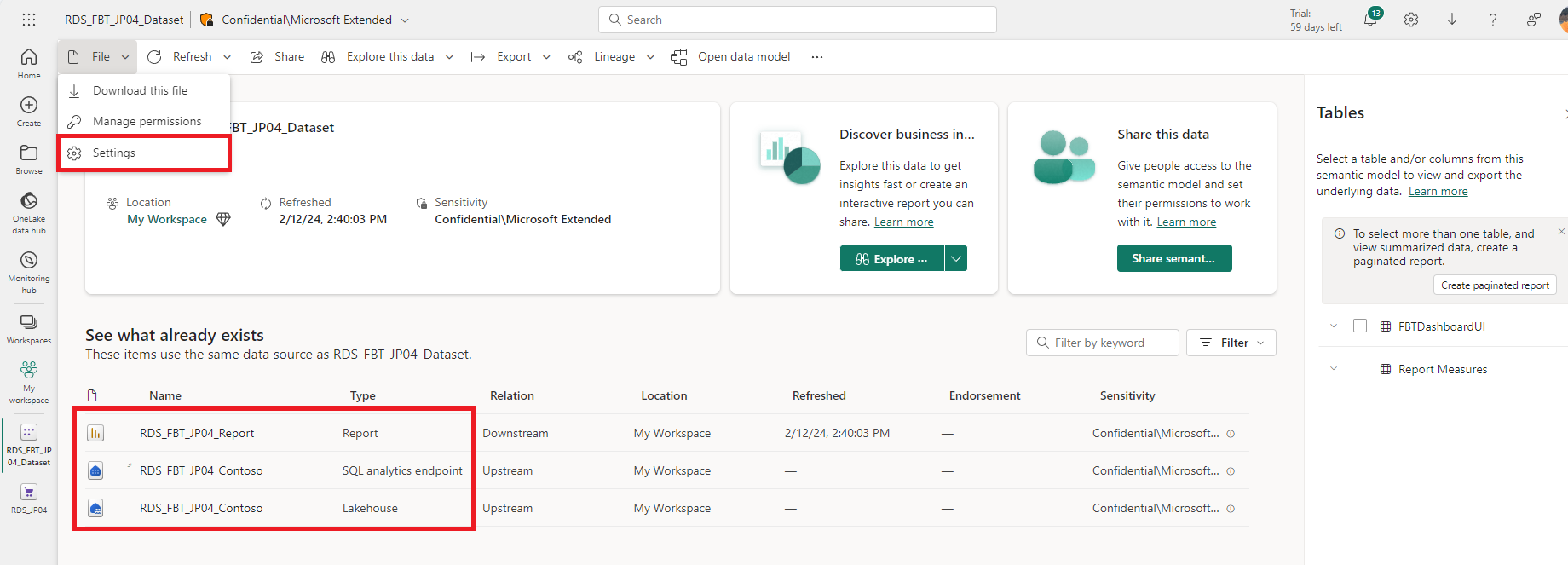
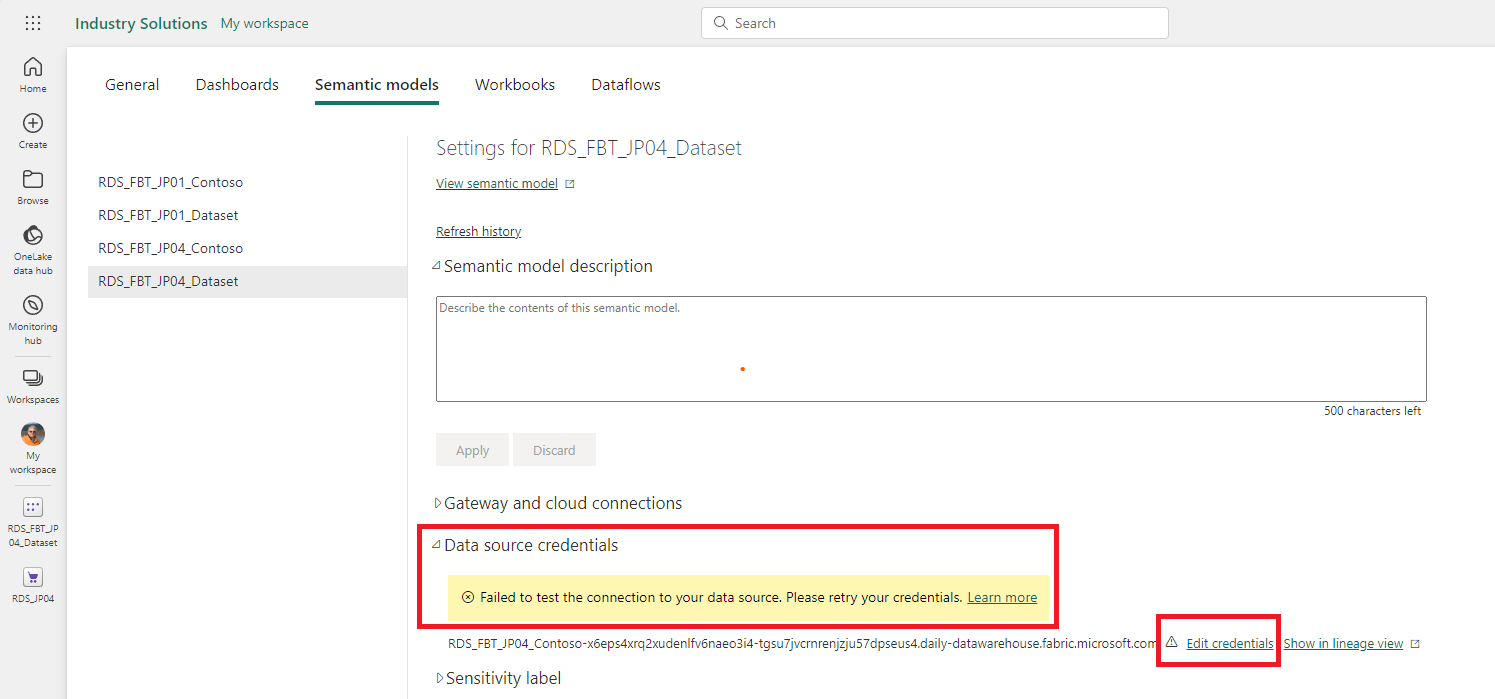
Select Semantic models tab. Under the Data source credentials section, there is an alert that says Failed to test the connection to your data source. Please retry your credentials. Select Edit credentials.
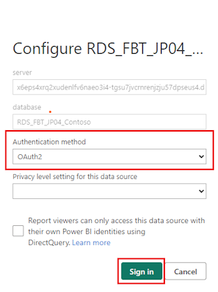
A popup window opens. Select OAuth2 as the authentication method, enter an optional privacy level, and select Sign in to sign in with this authentication.


Important
If you attempt to view the Frequently bought together report before configuring authentication for the dataset, you will see an error in the report window that says "An exception occurred due to an on-premise service issue".
Configure model to generate insights
The notebook consists of the following cells that tell the story of how data is processed to provide the required output.
Caution
The following cells are used in the specific sequence recommended. If they're used in a different sequence, the notebook fails.
1. Import libraries
This step imports the necessary libraries for the notebook. You don't have to make any changes in this step.
2. Initialize spark configs, logger, and checkpointer
This step initializes the spark configs, logger, and checkpointer objects that are used for the notebook execution.
The logger can be initialized in two different ways:
Set up to write logs to the notebook cell outputs. This behavior is the default.
Set up to write logs to an Azure Application Insights workspace, the connection_string of the Application Insights workspace would be needed. Also, a Run ID would be generated and shown in the cell's output and can be used to query logs in the Application Insights workspace.
The Checkpointer is used to synchronize Spark execution and to avoid potential generation of duplicated keys. You must provide a path that is used as a working directory. checkpoint_dir is the name of the variable. The directory must be within the files section of the Lakehouse. That is, it needs to start with "Files/".
3. Connect to Lakehouse and read input tables
This step connects to the Lakehouse and reads the input tables that are required for the model. The input tables are read from one of the three options listed:
The pinned Lakehouse of the notebook, which contains the sample data. This option is the default.
Any of the Lakehouses connected to the notebook. You can select the Lakehouse from a drop-down menu.
Another Lakehouse that isn't connected to the notebook. You need to provide the full path to the Lakehouse.
For details of input tables, see Input data for Frequently bought together.
The notebook allows you to run the model on multiple time periods, which can help you capture the seasonality and changes in customer behavior, product portfolio, and product positioning over time. You can also compare the results of different time periods using the out-of-the-box dashboard.
To define a time period, use the add_analysis_period function. Ensure to define the analysis periods within the duration of the input data. The duration of the input data (max and min transactions timestamp) is logged in the cell's output. You can define up to five time periods. The reference keys for the periods are stored in the TimePeriods table.
4. Preprocess input data
This step joins the input dataframes to create a POS dataset, which is used by the model to generate the insights. You don't have to make any changes in this step.
The output of this step is the following dataframes:
purchases: The purchases POS dataframe contains information about the purchases made by customers, such as, retail entity ID, product ID, product list price amount, quantity, and visit timestamp. This dataframe is created by joining the Visit, Order, Transaction, and TransactionLineItem tables.
time_periods: This dataframe contains the analysis periods defined by you in the previous step. These periods are used to split the data and run the model on each period.
retail_entities: This dataframe contains the retail entity IDs and their information. A retail entity can either be an individual store or a retailer. These entities are used to run the model on a store level or a retailer level.
5. Define model parameters and execute model
The following model parameters can be set to fine tune the model results:
Parameter name: min_itemset_frequency
Description: Minimal number of purchases of item sets (collection of two products bought together) to be considered in the analysis of the model.
Value type: integer
Default value: 3
Required: true.
Permitted values: >=1
Parameter name: max_basket_size
Description: Maximum number of items in one basket. If the number of items in the basket exceeds the default value, the basket is trimmed. The product with the lowest sales in the dataset is trimmed first.
Value type: integer
Default value: 20
Required: true.
Permitted values: >=1
Parameter name: chi_2_alpha
Description: Statistical significance parameter. Used to determine whether a pair of products associated together is meaningful and statistically significant. If a pair of products scores less than the parameter value, they're flagged in the Chi2IsSignificant field on the RuleAttributes table.
Value type: float
Required: false
Default value: 0.05 percentile
Permitted values range: 0-1
Upon execution, data is written to the output tables. You have three options to define which Lakehouse to write to.
6. Create Power BI dashboard tables
You can use the num_top_associated_products parameter to configure the number of top associated products to be displayed in the Power BI dashboard for each product.
Description: Maximum number of associated products for each product to be shown in the Power BI dashboard. Returns top products sorted by the CombinationRank field
Value type: integer
Required: false
Default value: 5
Permitted values range: 1-10
Upon execution, data is written to the Lakehouse. For details of output tables, see Output data for Frequently bought together.
Similar to the Connect to Lakehouse and read input tables section, there are three methods of writing outputs to Fabric.