你当前正在访问 Microsoft Azure Global Edition 技术文档网站。 如果需要访问由世纪互联运营的 Microsoft Azure 中国技术文档网站,请访问 https://docs.azure.cn。
本文介绍如何使用 Azure Quantum 资源估算器。 资源估算器可帮助你估算在量子计算机上运行量子程序所需的资源。 可以使用资源估算器来估算量子比特数、门数和运行量子程序所需的线路深度。
资源估算器在 Visual Studio Code 中与量子开发工具包扩展一起提供。 有关详细信息,请参阅 安装量子开发工具包。
警告
Azure 门户中的资源估算器已弃用。 建议转换到 Quantum 开发工具包中提供的 Visual Studio Code 中的本地资源估算器。
VS Code 的先决条件
- 最新版本的 Visual Studio Code 或打开网页版 VS Code。
- 最新版本的Quantum 开发工具包扩展。 有关安装详细信息,请参阅 设置 QDK 扩展。
提示
无需有 Azure 帐户即可运行资源估算器。
创建新的 Q# 文件
- 打开 Visual Studio Code 并选择“文件”>“新建文本文件”以创建新文件。
- 将文件另存为
ShorRE.qs。 此文件将包含程序的 Q# 代码。
创建量子算法
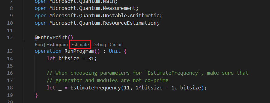
将以下代码复制到 ShorRE.qs 文件中:
    import Std.Arrays.*;
    import Std.Canon.*;
    import Std.Convert.*;
    import Std.Diagnostics.*;
    import Std.Math.*;
    import Std.Measurement.*;
    import Microsoft.Quantum.Unstable.Arithmetic.*;
    import Std.ResourceEstimation.*;

    operation Main() : Unit {
        let bitsize = 31;

        // When choosing parameters for `EstimateFrequency`, make sure that
        // generator and modules are not co-prime
        let _ = EstimateFrequency(11, 2^bitsize - 1, bitsize);
    }

    // In this sample we concentrate on costing the `EstimateFrequency`
    // operation, which is the core quantum operation in Shors algorithm, and
    // we omit the classical pre- and post-processing.

    /// # Summary
    /// Estimates the frequency of a generator
    /// in the residue ring Z mod `modulus`.
    ///
    /// # Input
    /// ## generator
    /// The unsigned integer multiplicative order (period)
    /// of which is being estimated. Must be co-prime to `modulus`.
    /// ## modulus
    /// The modulus which defines the residue ring Z mod `modulus`
    /// in which the multiplicative order of `generator` is being estimated.
    /// ## bitsize
    /// Number of bits needed to represent the modulus.
    ///
    /// # Output
    /// The numerator k of dyadic fraction k/2^bitsPrecision
    /// approximating s/r.
    operation EstimateFrequency(
        generator : Int,
        modulus : Int,
        bitsize : Int
    )
    : Int {
        mutable frequencyEstimate = 0;
        let bitsPrecision =  2 * bitsize + 1;

        // Allocate qubits for the superposition of eigenstates of
        // the oracle that is used in period finding.
        use eigenstateRegister = Qubit[bitsize];

        // Initialize eigenstateRegister to 1, which is a superposition of
        // the eigenstates we are estimating the phases of.
        // We first interpret the register as encoding an unsigned integer
        // in little endian encoding.
        ApplyXorInPlace(1, eigenstateRegister);
        let oracle = ApplyOrderFindingOracle(generator, modulus, _, _);

        // Use phase estimation with a semiclassical Fourier transform to
        // estimate the frequency.
        use c = Qubit();
        for idx in bitsPrecision - 1..-1..0 {
            within {
                H(c);
            } apply {
                // `BeginEstimateCaching` and `EndEstimateCaching` are the operations
                // exposed by Azure Quantum Resource Estimator. These will instruct
                // resource counting such that the if-block will be executed
                // only once, its resources will be cached, and appended in
                // every other iteration.
                if BeginEstimateCaching("ControlledOracle", SingleVariant()) {
                    Controlled oracle([c], (1 <<< idx, eigenstateRegister));
                    EndEstimateCaching();
                }
                R1Frac(frequencyEstimate, bitsPrecision - 1 - idx, c);
            }
            if MResetZ(c) == One {
                frequencyEstimate += 1 <<< (bitsPrecision - 1 - idx);
            }
        }

        // Return all the qubits used for oracles eigenstate back to 0 state
        // using Microsoft.Quantum.Intrinsic.ResetAll.
        ResetAll(eigenstateRegister);

        return frequencyEstimate;
    }

    /// # Summary
    /// Interprets `target` as encoding unsigned little-endian integer k
    /// and performs transformation |k⟩ ↦ |gᵖ⋅k mod N ⟩ where
    /// p is `power`, g is `generator` and N is `modulus`.
    ///
    /// # Input
    /// ## generator
    /// The unsigned integer multiplicative order ( period )
    /// of which is being estimated. Must be co-prime to `modulus`.
    /// ## modulus
    /// The modulus which defines the residue ring Z mod `modulus`
    /// in which the multiplicative order of `generator` is being estimated.
    /// ## power
    /// Power of `generator` by which `target` is multiplied.
    /// ## target
    /// Register interpreted as little endian encoded which is multiplied by
    /// given power of the generator. The multiplication is performed modulo
    /// `modulus`.
    internal operation ApplyOrderFindingOracle(
        generator : Int, modulus : Int, power : Int, target : Qubit[]
    )
    : Unit
    is Adj + Ctl {
        // The oracle we use for order finding implements |x⟩ ↦ |x⋅a mod N⟩. We
        // also use `ExpModI` to compute a by which x must be multiplied. Also
        // note that we interpret target as unsigned integer in little-endian
        // encoding.
        ModularMultiplyByConstant(modulus,
                                    ExpModI(generator, power, modulus),
                                    target);
    }

    /// # Summary
    /// Performs modular in-place multiplication by a classical constant.
    ///
    /// # Description
    /// Given the classical constants `c` and `modulus`, and an input
    /// quantum register  |𝑦⟩, this operation
    /// computes `(c*x) % modulus` into |𝑦⟩.
    ///
    /// # Input
    /// ## modulus
    /// Modulus to use for modular multiplication
    /// ## c
    /// Constant by which to multiply |𝑦⟩
    /// ## y
    /// Quantum register of target
    internal operation ModularMultiplyByConstant(modulus : Int, c : Int, y : Qubit[])
    : Unit is Adj + Ctl {
        use qs = Qubit[Length(y)];
        for (idx, yq) in Enumerated(y) {
            let shiftedC = (c <<< idx) % modulus;
            Controlled ModularAddConstant([yq], (modulus, shiftedC, qs));
        }
        ApplyToEachCA(SWAP, Zipped(y, qs));
        let invC = InverseModI(c, modulus);
        for (idx, yq) in Enumerated(y) {
            let shiftedC = (invC <<< idx) % modulus;
            Controlled ModularAddConstant([yq], (modulus, modulus - shiftedC, qs));
        }
    }

    /// # Summary
    /// Performs modular in-place addition of a classical constant into a
    /// quantum register.
    ///
    /// # Description
    /// Given the classical constants `c` and `modulus`, and an input
    /// quantum register  |𝑦⟩, this operation
    /// computes `(x+c) % modulus` into |𝑦⟩.
    ///
    /// # Input
    /// ## modulus
    /// Modulus to use for modular addition
    /// ## c
    /// Constant to add to |𝑦⟩
    /// ## y
    /// Quantum register of target
    internal operation ModularAddConstant(modulus : Int, c : Int, y : Qubit[])
    : Unit is Adj + Ctl {
        body (...) {
            Controlled ModularAddConstant([], (modulus, c, y));
        }
        controlled (ctrls, ...) {
            // We apply a custom strategy to control this operation instead of
            // letting the compiler create the controlled variant for us in which
            // the `Controlled` functor would be distributed over each operation
            // in the body.
            //
            // Here we can use some scratch memory to save ensure that at most one
            // control qubit is used for costly operations such as `AddConstant`
            // and `CompareGreaterThenOrEqualConstant`.
            if Length(ctrls) >= 2 {
                use control = Qubit();
                within {
                    Controlled X(ctrls, control);
                } apply {
                    Controlled ModularAddConstant([control], (modulus, c, y));
                }
            } else {
                use carry = Qubit();
                Controlled AddConstant(ctrls, (c, y + [carry]));
                Controlled Adjoint AddConstant(ctrls, (modulus, y + [carry]));
                Controlled AddConstant([carry], (modulus, y));
                Controlled CompareGreaterThanOrEqualConstant(ctrls, (c, y, carry));
            }
        }
    }

    /// # Summary
    /// Performs in-place addition of a constant into a quantum register.
    ///
    /// # Description
    /// Given a non-empty quantum register |𝑦⟩ of length 𝑛+1 and a positive
    /// constant 𝑐 < 2ⁿ, computes |𝑦 + c⟩ into |𝑦⟩.
    ///
    /// # Input
    /// ## c
    /// Constant number to add to |𝑦⟩.
    /// ## y
    /// Quantum register of second summand and target; must not be empty.
    internal operation AddConstant(c : Int, y : Qubit[]) : Unit is Adj + Ctl {
        // We are using this version instead of the library version that is based
        // on Fourier angles to show an advantage of sparse simulation in this sample.

        let n = Length(y);
        Fact(n > 0, "Bit width must be at least 1");

        Fact(c >= 0, "constant must not be negative");
        Fact(c < 2 ^ n, $"constant must be smaller than {2L ^ n}");

        if c != 0 {
            // If c has j trailing zeroes than the j least significant bits
            // of y won't be affected by the addition and can therefore be
            // ignored by applying the addition only to the other qubits and
            // shifting c accordingly.
            let j = NTrailingZeroes(c);
            use x = Qubit[n - j];
            within {
                ApplyXorInPlace(c >>> j, x);
            } apply {
                IncByLE(x, y[j...]);
            }
        }
    }

    /// # Summary
    /// Performs greater-than-or-equals comparison to a constant.
    ///
    /// # Description
    /// Toggles output qubit `target` if and only if input register `x`
    /// is greater than or equal to `c`.
    ///
    /// # Input
    /// ## c
    /// Constant value for comparison.
    /// ## x
    /// Quantum register to compare against.
    /// ## target
    /// Target qubit for comparison result.
    ///
    /// # Reference
    /// This construction is described in [Lemma 3, arXiv:2201.10200]
    internal operation CompareGreaterThanOrEqualConstant(c : Int, x : Qubit[], target : Qubit)
    : Unit is Adj+Ctl {
        let bitWidth = Length(x);

        if c == 0 {
            X(target);
        } elif c >= 2 ^ bitWidth {
            // do nothing
        } elif c == 2 ^ (bitWidth - 1) {
            ApplyLowTCNOT(Tail(x), target);
        } else {
            // normalize constant
            let l = NTrailingZeroes(c);

            let cNormalized = c >>> l;
            let xNormalized = x[l...];
            let bitWidthNormalized = Length(xNormalized);
            let gates = Rest(IntAsBoolArray(cNormalized, bitWidthNormalized));

            use qs = Qubit[bitWidthNormalized - 1];
            let cs1 = [Head(xNormalized)] + Most(qs);
            let cs2 = Rest(xNormalized);

            within {
                for i in IndexRange(gates) {
                    (gates[i] ? ApplyAnd | ApplyOr)(cs1[i], cs2[i], qs[i]);
                }
            } apply {
                ApplyLowTCNOT(Tail(qs), target);
            }
        }
    }

    /// # Summary
    /// Internal operation used in the implementation of GreaterThanOrEqualConstant.
    internal operation ApplyOr(control1 : Qubit, control2 : Qubit, target : Qubit) : Unit is Adj {
        within {
            ApplyToEachA(X, [control1, control2]);
        } apply {
            ApplyAnd(control1, control2, target);
            X(target);
        }
    }

    internal operation ApplyAnd(control1 : Qubit, control2 : Qubit, target : Qubit)
    : Unit is Adj {
        body (...) {
            CCNOT(control1, control2, target);
        }
        adjoint (...) {
            H(target);
            if (M(target) == One) {
                X(target);
                CZ(control1, control2);
            }
        }
    }


    /// # Summary
    /// Returns the number of trailing zeroes of a number
    ///
    /// ## Example
    /// ```qsharp
    /// let zeroes = NTrailingZeroes(21); // = NTrailingZeroes(0b1101) = 0
    /// let zeroes = NTrailingZeroes(20); // = NTrailingZeroes(0b1100) = 2
    /// ```
    internal function NTrailingZeroes(number : Int) : Int {
        mutable nZeroes = 0;
        mutable copy = number;
        while (copy % 2 == 0) {
            nZeroes += 1;
            copy /= 2;
        }
        return nZeroes;
    }

    /// # Summary
    /// An implementation for `CNOT` that when controlled using a single control uses
    /// a helper qubit and uses `ApplyAnd` to reduce the T-count to 4 instead of 7.
    internal operation ApplyLowTCNOT(a : Qubit, b : Qubit) : Unit is Adj+Ctl {
        body (...) {
            CNOT(a, b);
        }

        adjoint self;

        controlled (ctls, ...) {
            // In this application this operation is used in a way that
            // it is controlled by at most one qubit.
            Fact(Length(ctls) <= 1, "At most one control line allowed");

            if IsEmpty(ctls) {
                CNOT(a, b);
            } else {
                use q = Qubit();
                within {
                    ApplyAnd(Head(ctls), a, q);
                } apply {
                    CNOT(q, b);
                }
            }
        }

        controlled adjoint self;
    }
运行资源估算器
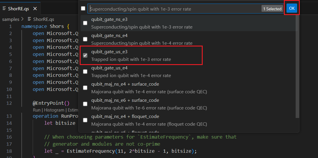
资源估算器提供 六个预定义的量子比特参数,其中四个具有基于入口的指令集,两个具有 Majorana 指令集。 它还提供两个 量子错误代码, surface_code 以及 floquet_code。
此示例中使用 qubit_gate_us_e3 量子比特参数和 surface_code 量子纠错代码运行资源估算器。
选择 “视图 -> 命令面板”,然后键入“resource”,应显示 Q#:计算资源估算 选项。 还可以单击”。 选择此选项可打开“资源估算器”窗口。
可以选择一个或多个“量子比特参数 + 纠错代码”类型来估算其资源。 对于此示例,选择“qubit_gate_us_e3”,然后单击“确定”。
指定“错误预算”或接受默认值 0.001。 对于此示例,请保留默认值,然后按 Enter。
按 Enter 接受基于文件名的默认结果名称,在本例中为 ShorRE。
查看结果
资源估算器为同一算法提供了多个估计值,每个算法都显示了量子比特数与运行时之间的权衡。 了解运行时和系统规模之间的权衡是资源估算的更重要方面之一。
资源估算的结果显示在“Q# 估算”窗口中。
“结果”选项卡显示资源估算的摘要。 单击第一行旁边的图标,选择要显示的列。 可以从运行名称、估计类型、量子比特类型、qec 方案、错误预算、逻辑量子比特、逻辑深度、代码距离、T 状态、T 工厂、T 工厂、T 工厂分数、运行时、rQOPS 和物理量子比特中进行选择。
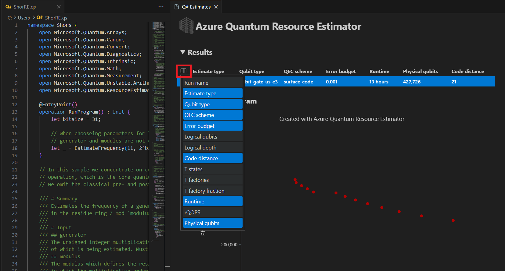
在结果表的“估计类型”列中,可以看到算法的 {量子比特数, 运行时} 的最佳组合数。 可以在时空图中查看这些组合。
空间图显示了物理量子比特数与算法运行时之间的权衡。 在这种情况下,资源估算器发现 13 种不同的最佳组合数千个可能的组合。 可以将鼠标悬停在每个 {数量的量子比特,运行时} 点上以查看该点的资源估算的详细信息。
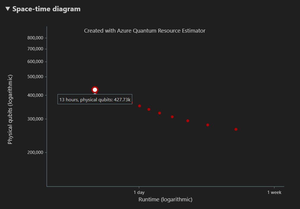
有关详细信息,请参阅 时空图。
注意
你需要 单击一个空间时间点 ,即 {数量的量子比特,运行时} 对,以查看空间关系图以及对应于该点的资源估算的详细信息。
空间图显示了用于算法的物理量子比特和 T 工厂的分布,对应于 {数量的量子比特,运行时} 对。 例如,如果在空间图中选择最左边的点,则运行算法所需的物理量子比特数427726,其中196686算法量子比特,其中 231040 个是 T 工厂量子比特。
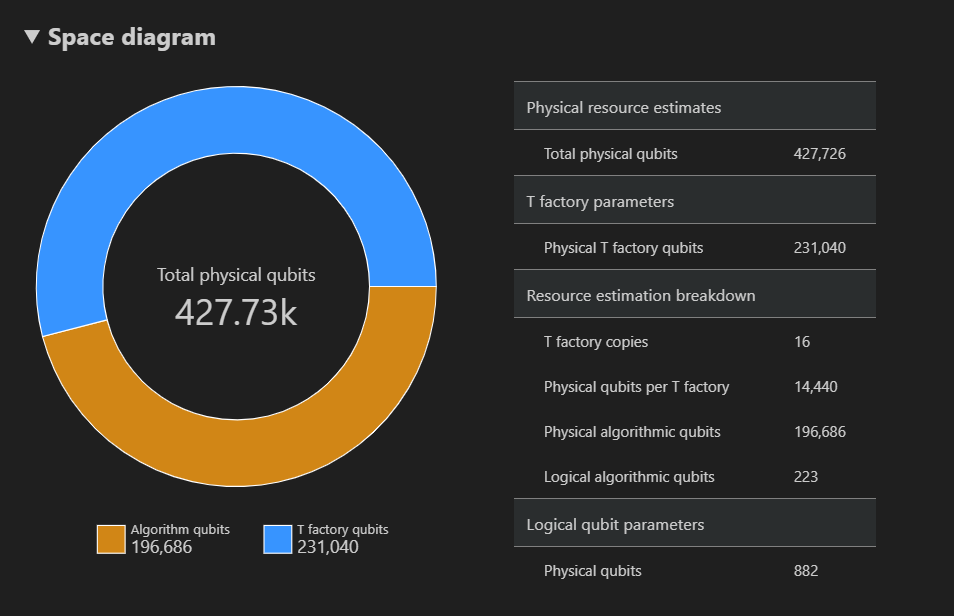
最后,“ 资源估算 ”选项卡显示与 {数量的量子比特、运行时} 对对应的资源估算器输出数据的完整列表。 可以通过折叠包含更多信息的组来检查成本详细信息。 例如,在空间关系图中选择最左侧的点,然后折叠 逻辑量子比特参数 组。
逻辑量子比特参数 值 QEC 方案 surface_code 码距 21 物理量子比特 882 逻辑周期时间 13 毫升 逻辑量子比特错误率 3.00E-13 交叉预制 0.03 错误更正阈值 0.01 逻辑周期时间公式 (4 * twoQubitGateTime+ 2 *oneQubitMeasurementTime) *codeDistance物理量子比特公式 2 * codeDistance*codeDistance提示
单击“显示详细行”可显示报表数据的每个输出的说明。
有关详细信息,请参阅 资源估算器的完整报表数据。
target更改参数
可以使用其他量子比特类型、更正代码和错误预算来估算同一 Q# 程序的成本。 通过选择“视图 -> 命令面板”打开“资源估算器”窗口,然后键入Q#: Calculate Resource Estimates。
选择任何其他配置,例如基于 Majorana 的量子比特参数 qubit_maj_ns_e6。 接受默认错误预算值或输入新值,然后按 Enter。 资源估算器使用新 target 参数重新运行估算。
有关详细信息,请参阅 Target 资源估算器的参数 。
运行多个参数配置
Azure Quantum 资源估算器可以运行多个参数配置 target ,并比较资源估算结果。
选择 视图 -> 命令面板,或按 Ctrl+Shift+P,然后键入
Q#: Calculate Resource Estimates。选择qubit_gate_us_e3、qubit_gate_us_e4、qubit_maj_ns_e4 + floquet_code,然后qubit_maj_ns_e6 + floquet_code,然后单击“确定”。
接受默认错误预算值 0.001,然后按 Enter。
按 Enter 接受输入文件,在本例中为 ShorRE.qs。
对于多个参数配置,结果将显示在“结果”选项卡中的不同行中。
空间图显示所有参数配置的结果。 结果表的第一列显示每个参数配置的图例。 可以将鼠标悬停在每个点上以查看该点的资源估算的详细信息。
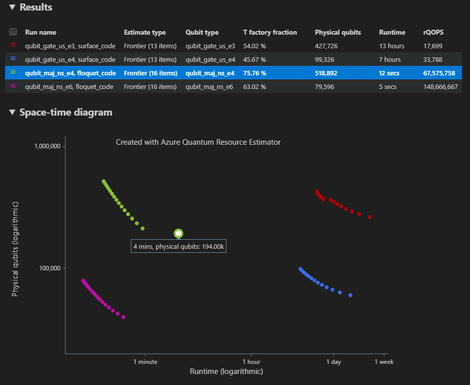
单击 空间图的 {数量的量子比特,运行时} 点 以显示相应的空间图和报告数据。
VS Code 中 Jupyter Notebook 的先决条件
安装了 Python 和 Pip 的 Python 环境。
最新版本的 Visual Studio Code 或打开网页版 VS Code。
安装了 Quantum 开发工具包、Python和 Jupyter 扩展的 VS Code。
最新的 Azure Quantum
qsharp和qsharp_widgets包。python -m pip install --upgrade qsharp qsharp_widgets或
!pip install --upgrade qsharp qsharp_widgets
提示
无需有 Azure 帐户即可运行资源估算器。
创建量子算法
在 VS Code 中,选择“视图 > 命令面板”,然后选择“创建:新 Jupyter Notebook”。
在右上角,VS Code 将检测并显示为笔记本选择的 Python 版本和虚拟 Python 环境。 如果有多个 Python 环境,可能需要使用右上角的内核选取器选择内核。 如果未检测到任何环境,请参阅 VS Code 中的 Jupyter Notebook 以获取设置信息。
在笔记本的第一个单元格中,导入
qsharp包。import qsharp添加新单元格并复制以下代码。
%%qsharp
import Std.Arrays.*;
import Std.Canon.*;
import Std.Convert.*;
import Std.Diagnostics.*;
import Std.Math.*;
import Std.Measurement.*;
import Microsoft.Quantum.Unstable.Arithmetic.*;
import Std.ResourceEstimation.*;

operation RunProgram() : Unit {
    let bitsize = 31;

    // When choosing parameters for `EstimateFrequency`, make sure that
    // generator and modules are not co-prime
    let _ = EstimateFrequency(11, 2^bitsize - 1, bitsize);
}


// In this sample we concentrate on costing the `EstimateFrequency`
// operation, which is the core quantum operation in Shors algorithm, and
// we omit the classical pre- and post-processing.

/// # Summary
/// Estimates the frequency of a generator
/// in the residue ring Z mod `modulus`.
///
/// # Input
/// ## generator
/// The unsigned integer multiplicative order (period)
/// of which is being estimated. Must be co-prime to `modulus`.
/// ## modulus
/// The modulus which defines the residue ring Z mod `modulus`
/// in which the multiplicative order of `generator` is being estimated.
/// ## bitsize
/// Number of bits needed to represent the modulus.
///
/// # Output
/// The numerator k of dyadic fraction k/2^bitsPrecision
/// approximating s/r.
operation EstimateFrequency(
    generator : Int,
    modulus : Int,
    bitsize : Int
)
: Int {
    mutable frequencyEstimate = 0;
    let bitsPrecision =  2 * bitsize + 1;

    // Allocate qubits for the superposition of eigenstates of
    // the oracle that is used in period finding.
    use eigenstateRegister = Qubit[bitsize];

    // Initialize eigenstateRegister to 1, which is a superposition of
    // the eigenstates we are estimating the phases of.
    // We first interpret the register as encoding an unsigned integer
    // in little endian encoding.
    ApplyXorInPlace(1, eigenstateRegister);
    let oracle = ApplyOrderFindingOracle(generator, modulus, _, _);

    // Use phase estimation with a semiclassical Fourier transform to
    // estimate the frequency.
    use c = Qubit();
    for idx in bitsPrecision - 1..-1..0 {
        within {
            H(c);
        } apply {
            // `BeginEstimateCaching` and `EndEstimateCaching` are the operations
            // exposed by Azure Quantum Resource Estimator. These will instruct
            // resource counting such that the if-block will be executed
            // only once, its resources will be cached, and appended in
            // every other iteration.
            if BeginEstimateCaching("ControlledOracle", SingleVariant()) {
                Controlled oracle([c], (1 <<< idx, eigenstateRegister));
                EndEstimateCaching();
            }
            R1Frac(frequencyEstimate, bitsPrecision - 1 - idx, c);
        }
        if MResetZ(c) == One {
            frequencyEstimate += 1 <<< (bitsPrecision - 1 - idx);
        }
    }

    // Return all the qubits used for oracle eigenstate back to 0 state
    // using Microsoft.Quantum.Intrinsic.ResetAll.
    ResetAll(eigenstateRegister);

    return frequencyEstimate;
}

/// # Summary
/// Interprets `target` as encoding unsigned little-endian integer k
/// and performs transformation |k⟩ ↦ |gᵖ⋅k mod N ⟩ where
/// p is `power`, g is `generator` and N is `modulus`.
///
/// # Input
/// ## generator
/// The unsigned integer multiplicative order ( period )
/// of which is being estimated. Must be co-prime to `modulus`.
/// ## modulus
/// The modulus which defines the residue ring Z mod `modulus`
/// in which the multiplicative order of `generator` is being estimated.
/// ## power
/// Power of `generator` by which `target` is multiplied.
/// ## target
/// Register interpreted as little endian encoded which is multiplied by
/// given power of the generator. The multiplication is performed modulo
/// `modulus`.
internal operation ApplyOrderFindingOracle(
    generator : Int, modulus : Int, power : Int, target : Qubit[]
)
: Unit
is Adj + Ctl {
    // The oracle we use for order finding implements |x⟩ ↦ |x⋅a mod N⟩. We
    // also use `ExpModI` to compute a by which x must be multiplied. Also
    // note that we interpret target as unsigned integer in little-endian
    // encoding.
    ModularMultiplyByConstant(modulus,
                                ExpModI(generator, power, modulus),
                                target);
}

/// # Summary
/// Performs modular in-place multiplication by a classical constant.
///
/// # Description
/// Given the classical constants `c` and `modulus`, and an input
/// quantum register |𝑦⟩, this operation
/// computes `(c*x) % modulus` into |𝑦⟩.
///
/// # Input
/// ## modulus
/// Modulus to use for modular multiplication
/// ## c
/// Constant by which to multiply |𝑦⟩
/// ## y
/// Quantum register of target
internal operation ModularMultiplyByConstant(modulus : Int, c : Int, y : Qubit[])
: Unit is Adj + Ctl {
    use qs = Qubit[Length(y)];
    for (idx, yq) in Enumerated(y) {
        let shiftedC = (c <<< idx) % modulus;
        Controlled ModularAddConstant([yq], (modulus, shiftedC, qs));
    }
    ApplyToEachCA(SWAP, Zipped(y, qs));
    let invC = InverseModI(c, modulus);
    for (idx, yq) in Enumerated(y) {
        let shiftedC = (invC <<< idx) % modulus;
        Controlled ModularAddConstant([yq], (modulus, modulus - shiftedC, qs));
    }
}

/// # Summary
/// Performs modular in-place addition of a classical constant into a
/// quantum register.
///
/// # Description
/// Given the classical constants `c` and `modulus`, and an input
/// quantum register  |𝑦⟩, this operation
/// computes `(x+c) % modulus` into |𝑦⟩.
///
/// # Input
/// ## modulus
/// Modulus to use for modular addition
/// ## c
/// Constant to add to |𝑦⟩
/// ## y
/// Quantum register of target
internal operation ModularAddConstant(modulus : Int, c : Int, y : Qubit[])
: Unit is Adj + Ctl {
    body (...) {
        Controlled ModularAddConstant([], (modulus, c, y));
    }
    controlled (ctrls, ...) {
        // We apply a custom strategy to control this operation instead of
        // letting the compiler create the controlled variant for us in which
        // the `Controlled` functor would be distributed over each operation
        // in the body.
        //
        // Here we can use some scratch memory to save ensure that at most one
        // control qubit is used for costly operations such as `AddConstant`
        // and `CompareGreaterThenOrEqualConstant`.
        if Length(ctrls) >= 2 {
            use control = Qubit();
            within {
                Controlled X(ctrls, control);
            } apply {
                Controlled ModularAddConstant([control], (modulus, c, y));
            }
        } else {
            use carry = Qubit();
            Controlled AddConstant(ctrls, (c, y + [carry]));
            Controlled Adjoint AddConstant(ctrls, (modulus, y + [carry]));
            Controlled AddConstant([carry], (modulus, y));
            Controlled CompareGreaterThanOrEqualConstant(ctrls, (c, y, carry));
        }
    }
}

/// # Summary
/// Performs in-place addition of a constant into a quantum register.
///
/// # Description
/// Given a non-empty quantum register |𝑦⟩ of length 𝑛+1 and a positive
/// constant 𝑐 < 2ⁿ, computes |𝑦 + c⟩ into |𝑦⟩.
///
/// # Input
/// ## c
/// Constant number to add to |𝑦⟩.
/// ## y
/// Quantum register of second summand and target; must not be empty.
internal operation AddConstant(c : Int, y : Qubit[]) : Unit is Adj + Ctl {
    // We are using this version instead of the library version that is based
    // on Fourier angles to show an advantage of sparse simulation in this sample.

    let n = Length(y);
    Fact(n > 0, "Bit width must be at least 1");

    Fact(c >= 0, "constant must not be negative");
    Fact(c < 2 ^ n, $"constant must be smaller than {2L ^ n}");

    if c != 0 {
        // If c has j trailing zeroes than the j least significant bits
        // of y will not be affected by the addition and can therefore be
        // ignored by applying the addition only to the other qubits and
        // shifting c accordingly.
        let j = NTrailingZeroes(c);
        use x = Qubit[n - j];
        within {
            ApplyXorInPlace(c >>> j, x);
        } apply {
            IncByLE(x, y[j...]);
        }
    }
}

/// # Summary
/// Performs greater-than-or-equals comparison to a constant.
///
/// # Description
/// Toggles output qubit `target` if and only if input register `x`
/// is greater than or equal to `c`.
///
/// # Input
/// ## c
/// Constant value for comparison.
/// ## x
/// Quantum register to compare against.
/// ## target
/// Target qubit for comparison result.
///
/// # Reference
/// This construction is described in [Lemma 3, arXiv:2201.10200]
internal operation CompareGreaterThanOrEqualConstant(c : Int, x : Qubit[], target : Qubit)
: Unit is Adj+Ctl {
    let bitWidth = Length(x);

    if c == 0 {
        X(target);
    } elif c >= 2 ^ bitWidth {
        // do nothing
    } elif c == 2 ^ (bitWidth - 1) {
        ApplyLowTCNOT(Tail(x), target);
    } else {
        // normalize constant
        let l = NTrailingZeroes(c);

        let cNormalized = c >>> l;
        let xNormalized = x[l...];
        let bitWidthNormalized = Length(xNormalized);
        let gates = Rest(IntAsBoolArray(cNormalized, bitWidthNormalized));

        use qs = Qubit[bitWidthNormalized - 1];
        let cs1 = [Head(xNormalized)] + Most(qs);
        let cs2 = Rest(xNormalized);

        within {
            for i in IndexRange(gates) {
                (gates[i] ? ApplyAnd | ApplyOr)(cs1[i], cs2[i], qs[i]);
            }
        } apply {
            ApplyLowTCNOT(Tail(qs), target);
        }
    }
}

/// # Summary
/// Internal operation used in the implementation of GreaterThanOrEqualConstant.
internal operation ApplyOr(control1 : Qubit, control2 : Qubit, target : Qubit) : Unit is Adj {
    within {
        ApplyToEachA(X, [control1, control2]);
    } apply {
        ApplyAnd(control1, control2, target);
        X(target);
    }
}

internal operation ApplyAnd(control1 : Qubit, control2 : Qubit, target : Qubit)
: Unit is Adj {
    body (...) {
        CCNOT(control1, control2, target);
    }
    adjoint (...) {
        H(target);
        if (M(target) == One) {
            X(target);
            CZ(control1, control2);
        }
    }
}


/// # Summary
/// Returns the number of trailing zeroes of a number
///
/// ## Example
/// ```qsharp
/// let zeroes = NTrailingZeroes(21); // = NTrailingZeroes(0b1101) = 0
/// let zeroes = NTrailingZeroes(20); // = NTrailingZeroes(0b1100) = 2
/// ```
internal function NTrailingZeroes(number : Int) : Int {
    mutable nZeroes = 0;
    mutable copy = number;
    while (copy % 2 == 0) {
        nZeroes += 1;
        copy /= 2;
    }
    return nZeroes;
}

/// # Summary
/// An implementation for `CNOT` that when controlled using a single control uses
/// a helper qubit and uses `ApplyAnd` to reduce the T-count to 4 instead of 7.
internal operation ApplyLowTCNOT(a : Qubit, b : Qubit) : Unit is Adj+Ctl {
    body (...) {
        CNOT(a, b);
    }

    adjoint self;

    controlled (ctls, ...) {
        // In this application this operation is used in a way that
        // it is controlled by at most one qubit.
        Fact(Length(ctls) <= 1, "At most one control line allowed");

        if IsEmpty(ctls) {
            CNOT(a, b);
        } else {
            use q = Qubit();
            within {
                ApplyAnd(Head(ctls), a, q);
            } apply {
                CNOT(q, b);
            }
        }
    }

    controlled adjoint self;
}
估计量子算法
现在使用默认假设来估算 RunProgram 操作的物理资源。 添加新单元格并复制以下代码。
result = qsharp.estimate("RunProgram()")
result
qsharp.estimate 函数创建一个结果对象,可用于显示整体物理资源计数的表。 可以通过展开包含更多信息的组来查看成本详情。 有关详细信息,请参阅 资源估算器的完整报表数据。
例如,展开逻辑量子比特参数组,可以发现代码距离为 21,物理量子比特数为 882。
| 逻辑量子比特参数 | 值 |
|---|---|
| QEC 方案 | surface_code |
| 码距 | 21 |
| 物理量子比特 | 882 |
| 逻辑周期时间 | 8 毫升 |
| 逻辑量子比特错误率 | 3.00E-13 |
| 交叉预制 | 0.03 |
| 错误更正阈值 | 0.01 |
| 逻辑周期时间公式 | (4 * twoQubitGateTime + 2 * oneQubitMeasurementTime) * codeDistance |
| 物理量子比特公式 | 2 * codeDistance * codeDistance |
提示
对于更紧凑的输出表,可以使用 result.summary。
空间图
用于算法和 T 工厂的物理量子比特的分布可能会影响算法设计。 可以使用 qsharp-widgets 包来可视化此分布,以便更好地了解算法的预计空间要求。
from qsharp-widgets import SpaceChart, EstimateDetails
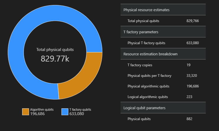
SpaceChart(result)
在此示例中,运行算法所需的物理量子比特数为 829766,其中 196686 个是算法量子比特,633080 个是 T 工厂量子比特。
更改默认值并估计算法
为程序提交资源估算请求时,可以指定一些可选参数。 使用 jobParams 字段访问可传递给作业执行的所有 target 参数,并查看假定的默认值:
result['jobParams']
{'errorBudget': 0.001,
 'qecScheme': {'crossingPrefactor': 0.03,
  'errorCorrectionThreshold': 0.01,
  'logicalCycleTime': '(4 * twoQubitGateTime + 2 * oneQubitMeasurementTime) * codeDistance',
  'name': 'surface_code',
  'physicalQubitsPerLogicalQubit': '2 * codeDistance * codeDistance'},
 'qubitParams': {'instructionSet': 'GateBased',
  'name': 'qubit_gate_ns_e3',
  'oneQubitGateErrorRate': 0.001,
  'oneQubitGateTime': '50 ns',
  'oneQubitMeasurementErrorRate': 0.001,
  'oneQubitMeasurementTime': '100 ns',
  'tGateErrorRate': 0.001,
  'tGateTime': '50 ns',
  'twoQubitGateErrorRate': 0.001,
  'twoQubitGateTime': '50 ns'}}
可以看到,资源估算器采用了 qubit_gate_ns_e3 量子比特模型、surface_code 纠错代码和 0.001 错误预算作为估算的默认值。
以下是 target 可以自定义的参数:
errorBudget- 算法的总体允许错误预算qecScheme- 量子纠错 (QEC) 方案qubitParams- 物理量子比特参数constraints- 组件级约束distillationUnitSpecifications- T 工厂蒸馏算法的规范estimateType- 单一或边界
有关详细信息,请参阅 Target 资源估算器的参数 。
更改量子比特模型
可以使用基于 Majorana 的量子比特参数 qubitParams“qubit_maj_ns_e6”估算同一算法的成本。
result_maj = qsharp.estimate("RunProgram()", params={
                "qubitParams": {
                    "name": "qubit_maj_ns_e6"
                }})
EstimateDetails(result_maj)
更改量子纠错方案
对于基于 Majorana 的量子比特参数上的同一示例,可以使用已 floque 的 QEC 方案 qecScheme 重新运行资源估算作业。
result_maj = qsharp.estimate("RunProgram()", params={
                "qubitParams": {
                    "name": "qubit_maj_ns_e6"
                },
                "qecScheme": {
                    "name": "floquet_code"
                }})
EstimateDetails(result_maj)
更改错误预算
接下来,使用 10% 的 errorBudget 重新运行同一量子线路。
result_maj = qsharp.estimate("RunProgram()", params={
                "qubitParams": {
                    "name": "qubit_maj_ns_e6"
                },
                "qecScheme": {
                    "name": "floquet_code"
                },
                "errorBudget": 0.1})
EstimateDetails(result_maj)
使用资源估算器进行批处理
Azure Quantum 资源估算器允许运行多个参数配置 target ,并比较结果。 如果要比较不同量子比特模型、QEC 方案或错误预算的成本,这会非常有用。
可以通过将参数target列表
params传递给函数的参数qsharp.estimate来执行批处理估计。 例如,使用默认参数和基于 Majorana 的量子比特参数运行同一算法,并使用 floquet QEC 方案。result_batch = qsharp.estimate("RunProgram()", params= [{}, # Default parameters { "qubitParams": { "name": "qubit_maj_ns_e6" }, "qecScheme": { "name": "floquet_code" } }]) result_batch.summary_data_frame(labels=["Gate-based ns, 10⁻³", "Majorana ns, 10⁻⁶"])型号 逻辑量子比特 逻辑深度 T 状态 码距 T 工厂 T 工厂分数 物理量子比特 rQOPS 物理运行时 基于门的 ns,10⁻³ 223 3.64M 4.70M 21 19 76.30 % 829.77k 26.55M 31 秒 Majorana ns,10⁻⁶ 223 3.64M 4.70M 5 19 63.02 % 79.60k 148.67M 5 秒 还可以使用
EstimatorParams类构造估计参数列表。from qsharp.estimator import EstimatorParams, QubitParams, QECScheme, LogicalCounts labels = ["Gate-based µs, 10⁻³", "Gate-based µs, 10⁻⁴", "Gate-based ns, 10⁻³", "Gate-based ns, 10⁻⁴", "Majorana ns, 10⁻⁴", "Majorana ns, 10⁻⁶"] params = EstimatorParams(num_items=6) params.error_budget = 0.333 params.items[0].qubit_params.name = QubitParams.GATE_US_E3 params.items[1].qubit_params.name = QubitParams.GATE_US_E4 params.items[2].qubit_params.name = QubitParams.GATE_NS_E3 params.items[3].qubit_params.name = QubitParams.GATE_NS_E4 params.items[4].qubit_params.name = QubitParams.MAJ_NS_E4 params.items[4].qec_scheme.name = QECScheme.FLOQUET_CODE params.items[5].qubit_params.name = QubitParams.MAJ_NS_E6 params.items[5].qec_scheme.name = QECScheme.FLOQUET_CODEqsharp.estimate("RunProgram()", params=params).summary_data_frame(labels=labels)型号 逻辑量子比特 逻辑深度 T 状态 码距 T 工厂 T 工厂分数 物理量子比特 rQOPS 物理运行时 基于门的 µs,10⁻³ 223 3.64M 4.70M 17 13 40.54% 216.77k 21.86k 10 小时 基于门的 µs,10⁻⁴ 223 3.64M 4.70M 9 14 43.17% 63.57k 41.30k 5 小时 基于门的 ns,10⁻³ 223 3.64M 4.70M 17 16 69.08% 416.89k 32.79M 25 秒 基于门的 ns,10⁻⁴ 223 3.64M 4.70M 9 14 43.17% 63.57k 61.94M 13 秒 Majorana ns,10⁻⁴ 223 3.64M 4.70M 9 19 82.75% 501.48k 82.59M 10 秒 Majorana ns,10⁻⁶ 223 3.64M 4.70M 5 13 31.47% 42.96k 148.67M 5 秒
运行 Pareto 边界估计
估算算法的资源时,请务必考虑物理量子比特数与算法运行时之间的权衡。 可以考虑分配尽可能多的物理量子比特以减少算法的运行时。 但是,物理量子比特的数量受量子硬件中可用的物理量子比特数的限制。
Pareto 边界估计为同一算法提供了多个估计值,每个算法在量子比特数和运行时之间进行权衡。
若要使用 Pareto 边界估计运行资源估算器,需要将参数指定
"estimateType"target 为"frontier"。 例如,使用 Pareto 边界估计,使用基于 Majorana 的量子比特参数运行同一算法,并使用图面代码。result = qsharp.estimate("RunProgram()", params= {"qubitParams": { "name": "qubit_maj_ns_e4" }, "qecScheme": { "name": "surface_code" }, "estimateType": "frontier", # frontier estimation } )可以使用函数
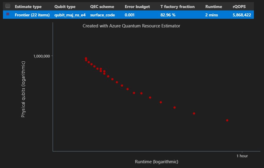
EstimatesOverview显示具有整体物理资源计数的表。 单击第一行旁边的图标,选择要显示的列。 可以从运行名称、估计类型、量子比特类型、qec 方案、错误预算、逻辑量子比特、逻辑深度、代码距离、T 状态、T 工厂、T 工厂、T 工厂分数、运行时、rQOPS 和物理量子比特中进行选择。from qsharp_widgets import EstimatesOverview EstimatesOverview(result)
在 结果表的“估计类型 ”列中,可以看到算法的 {量子比特数, 运行时} 的不同组合数。 在这种情况下,资源估算器发现 22 个不同的最佳组合数千个可能的组合。
时空关系图
该 EstimatesOverview 函数还显示 资源估算器的时空关系图 。
空间时间关系图显示每个 {量子比特数, 运行时} 对的物理量子比特数和算法的运行时。 可以将鼠标悬停在每个点上以查看该点的资源估算的详细信息。
使用 Pareto 边界估计进行批处理
若要估算和比较多个参数配置 target 与边界估计,请添加到
"estimateType": "frontier",参数中。result = qsharp.estimate( "RunProgram()", [ { "qubitParams": { "name": "qubit_maj_ns_e4" }, "qecScheme": { "name": "surface_code" }, "estimateType": "frontier", # Pareto frontier estimation }, { "qubitParams": { "name": "qubit_maj_ns_e6" }, "qecScheme": { "name": "floquet_code" }, "estimateType": "frontier", # Pareto frontier estimation }, ] ) EstimatesOverview(result, colors=["#1f77b4", "#ff7f0e"], runNames=["e4 Surface Code", "e6 Floquet Code"])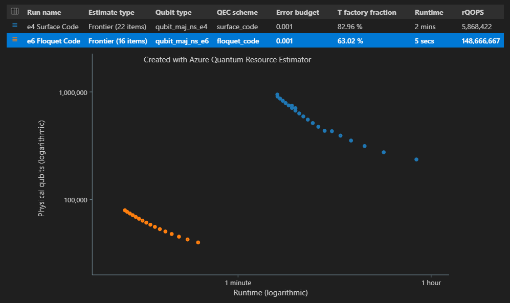
注意
可以使用函数
EstimatesOverview定义量子比特时间关系图的颜色和运行名称。使用 Pareto 边界估计运行多个参数配置 target 时,可以看到空间图的特定时间点的资源估计值,即每个 {量子比特数、运行时} 对。 例如,以下代码显示第二个(estimate index=0)运行和第四个(point index=3)最短运行时的估计详细信息使用情况。
EstimateDetails(result[1], 4)还可以查看空间图中特定时间点的空间关系图。 例如,以下代码显示了第一次运行组合(估计索引=0)和第三个最短运行时(点索引=2)的空间图。
SpaceChart(result[0], 2)
在 VS Code 中使用 Qiskit 的先决条件
安装了 Python 和 Pip 的 Python 环境。
最新版本的 Visual Studio Code 或打开 Web 的 Visual Studio Code。
安装了 Quantum 开发工具包、Python和 Jupyter 扩展的 VS Code。
最新的 Azure Quantum
qsharp和qsharp_widgets,以及qiskit包。python -m pip install --upgrade qsharp qsharp_widgets qiskit或
!pip install --upgrade qsharp qsharp_widgets qiskit
提示
无需有 Azure 帐户即可运行资源估算器。
创建新的 Jupyter Notebook
- 在 VS Code 中,选择“视图 > 命令面板”,然后选择“创建:新 Jupyter Notebook”。
- 在右上角,VS Code 将检测并显示为笔记本选择的 Python 版本和虚拟 Python 环境。 如果有多个 Python 环境,可能需要使用右上角的内核选取器选择内核。 如果未检测到任何环境,请参阅 VS Code 中的 Jupyter Notebook 以获取设置信息。
创建量子算法
在此示例中,将基于 Ruiz-Perez 和 Garcia-Escartin(arXiv:1411.5949)中显示的 构造(使用 Quantum Fourier Transform 实现算术) 为乘数创建量子线路。
可以通过更改 bitwidth 变量来调整乘数的大小。 线路生成包装在可以使用乘数值调用 bitwidth 的函数中。 该操作将有两个输入寄存器,每个输入寄存器的大小指定 bitwidth,一个输出寄存器是指定 bitwidth大小的两倍。 该函数还将输出直接从量子线路中提取的乘数的一些逻辑资源计数。
from qiskit.circuit.library import RGQFTMultiplier

def create_algorithm(bitwidth):
    print(f"[INFO] Create a QFT-based multiplier with bitwidth {bitwidth}")

    circ = RGQFTMultiplier(num_state_qubits=bitwidth)

    return circ
注意
如果选择 Python 内核并且无法识别 qiskit 模块,请尝试在内核选取器中选择其他 Python 环境。
估计量子算法
使用 create_algorithm 函数创建算法的实例。 可以通过更改 bitwidth 变量来调整乘数的大小。
bitwidth = 4

circ = create_algorithm(bitwidth)
使用默认假设估算此操作的物理资源。 可以使用 estimate 调用,该调用被重载以接受 Qiskit 的 QuantumCircuit 对象。
from qsharp.estimator import EstimatorParams
from qsharp.interop.qiskit import estimate

params = EstimatorParams()
result = estimate(circ, params)
或者,您可以使用 ResourceEstimatorBackend 来执行估算,正如现有的后端所做的那样。
from qsharp.interop.qiskit import ResourceEstimatorBackend
from qsharp.estimator import EstimatorParams

params = EstimatorParams()
backend = ResourceEstimatorBackend()

job = backend.run(circ, params)
result = job.result()
result 对象包含资源估算作业的输出。 可以使用 EstimateDetails 函数以更可读的格式显示结果。
from qsharp_widgets import EstimateDetails
EstimateDetails(result)
EstimateDetails 函数显示一个包含总体物理资源计数的表。 可以通过展开包含更多信息的组来查看成本详情。 有关详细信息,请参阅 资源估算器的完整报表数据。
例如,如果展开逻辑量子比特参数组,则可以更轻松地发现错误更正代码距离为 15。
| 逻辑量子比特参数 | 值 |
|---|---|
| QEC 方案 | surface_code |
| 码距 | 15 |
| 物理量子比特 | 450 |
| 逻辑周期时间 | 6us |
| 逻辑量子比特错误率 | 3.00E-10 |
| 交叉预制 | 0.03 |
| 错误更正阈值 | 0.01 |
| 逻辑周期时间公式 | (4 * twoQubitGateTime + 2 * oneQubitMeasurementTime) * codeDistance |
| 物理量子比特公式 | 2 * codeDistance * codeDistance |
在 物理量子比特参数 组中,可以看到假定用于此估计的物理量子比特属性。 例如,执行单量子比特测量和单量子比特门的时间分别假设为 100 ns 和 50 ns。
提示
还可以使用 result.data() 方法以 Python 字典的形式访问资源估算器的输出。 例如,访问物理计数 result.data()["physicalCounts"]。
空间图
用于算法和 T 工厂的物理量子比特的分布可能会影响算法设计。 可以将此分布可视化,以便更好地了解算法的估计空间要求。
from qsharp_widgets import SpaceChart

SpaceChart(result)
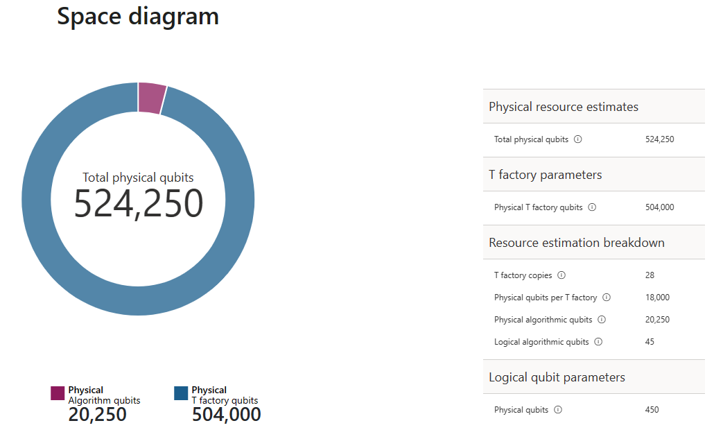
空间图显示了算法量子比特和 T 工厂量子比特的比例。 请注意,T 工厂副本数(19 个)对 T 工厂的物理量子比特数的贡献为$\text{T 工厂} \cdot \text{每个 T 工厂的物理量子比特数}= 19 \cdot 18,000 = 342,000$。
有关详细信息,请参阅 T 工厂物理估计。
更改默认值并估计算法
为程序提交资源估算请求时,可以指定一些可选参数。 使用 jobParams 字段访问可传递给作业执行的所有值,并查看假定的默认值:
result.data()["jobParams"]
{'errorBudget': 0.001,
 'qecScheme': {'crossingPrefactor': 0.03,
  'errorCorrectionThreshold': 0.01,
  'logicalCycleTime': '(4 * twoQubitGateTime + 2 * oneQubitMeasurementTime) * codeDistance',
  'name': 'surface_code',
  'physicalQubitsPerLogicalQubit': '2 * codeDistance * codeDistance'},
 'qubitParams': {'instructionSet': 'GateBased',
  'name': 'qubit_gate_ns_e3',
  'oneQubitGateErrorRate': 0.001,
  'oneQubitGateTime': '50 ns',
  'oneQubitMeasurementErrorRate': 0.001,
  'oneQubitMeasurementTime': '100 ns',
  'tGateErrorRate': 0.001,
  'tGateTime': '50 ns',
  'twoQubitGateErrorRate': 0.001,
  'twoQubitGateTime': '50 ns'}}
以下是 target 可以自定义的参数:
errorBudget- 总体允许的错误预算qecScheme- 量子纠错 (QEC) 方案qubitParams- 物理量子比特参数constraints- 组件级约束distillationUnitSpecifications- T 工厂蒸馏算法的规范
有关详细信息,请参阅 Target 资源估算器的参数 。
更改量子比特模型
接下来,使用基于 Majorana 的量子比特参数估算同一算法的成本 qubit_maj_ns_e6
qubitParams = {
    "name": "qubit_maj_ns_e6"
}

result = backend.run(circ, qubitParams).result()
可以编程方式检查物理计数。 例如,可以浏览有关创建以执行算法的 T 工厂的详细信息。
result.data()["tfactory"]
{'eccDistancePerRound': [1, 1, 5],
 'logicalErrorRate': 1.6833177305222897e-10,
 'moduleNamePerRound': ['15-to-1 space efficient physical',
  '15-to-1 RM prep physical',
  '15-to-1 RM prep logical'],
 'numInputTstates': 20520,
 'numModulesPerRound': [1368, 20, 1],
 'numRounds': 3,
 'numTstates': 1,
 'physicalQubits': 16416,
 'physicalQubitsPerRound': [12, 31, 1550],
 'runtime': 116900.0,
 'runtimePerRound': [4500.0, 2400.0, 110000.0]}
注意
默认情况下,运行时以纳秒为单位显示。
可以使用此数据生成一些说明,说明 T 工厂如何生成所需的 T 状态。
data = result.data()
tfactory = data["tfactory"]
breakdown = data["physicalCounts"]["breakdown"]
producedTstates = breakdown["numTfactories"] * breakdown["numTfactoryRuns"] * tfactory["numTstates"]

print(f"""A single T factory produces {tfactory["logicalErrorRate"]:.2e} T states with an error rate of (required T state error rate is {breakdown["requiredLogicalTstateErrorRate"]:.2e}).""")
print(f"""{breakdown["numTfactories"]} copie(s) of a T factory are executed {breakdown["numTfactoryRuns"]} time(s) to produce {producedTstates} T states ({breakdown["numTstates"]} are required by the algorithm).""")
print(f"""A single T factory is composed of {tfactory["numRounds"]} rounds of distillation:""")
for round in range(tfactory["numRounds"]):
    print(f"""- {tfactory["numUnitsPerRound"][round]} {tfactory["unitNamePerRound"][round]} unit(s)""")
A single T factory produces 1.68e-10 T states with an error rate of (required T state error rate is 2.77e-08).
23 copies of a T factory are executed 523 time(s) to produce 12029 T states (12017 are required by the algorithm).
A single T factory is composed of 3 rounds of distillation:
- 1368 15-to-1 space efficient physical unit(s)
- 20 15-to-1 RM prep physical unit(s)
- 1 15-to-1 RM prep logical unit(s)
更改量子纠错方案
现在,使用软盘 QEC 方案 qecScheme重新运行基于 Majorana 的量子比特参数上的同一示例的资源估算作业。
params = {
    "qubitParams": {"name": "qubit_maj_ns_e6"},
    "qecScheme": {"name": "floquet_code"}
}

result_maj_floquet = backend.run(circ, params).result()
EstimateDetails(result_maj_floquet)
更改错误预算
让我们重新运行一个 10% 的同一 errorBudget 量子线路。
params = {
    "errorBudget": 0.01,
    "qubitParams": {"name": "qubit_maj_ns_e6"},
    "qecScheme": {"name": "floquet_code"},
}
result_maj_floquet_e1 = backend.run(circ, params).result()
EstimateDetails(result_maj_floquet_e1)
注意
如果在使用资源估算器时遇到任何问题,请查看 “故障排除”页或联系 AzureQuantumInfo@microsoft.com。