本教程展示了数据科学工作流程的端到端示例。 该场景通过利用基于历史数据训练的机器学习算法构建欺诈检测模型。 然后,它使用模型来检测未来的欺诈交易。
本教程介绍以下步骤:
- 安装自定义库
- 加载数据
- 通过探索性数据分析了解和处理数据
- 使用 scikit-learn 训练机器学习模型,并使用 MLflow 和 Fabric 自动记录功能跟踪实验
- 保存并注册性能最高的machine learning模型
- 加载用于评分和进行预测的machine learning模型
先决条件
获取 Microsoft Fabric 订阅。 或者,注册免费的 Microsoft Fabric 试用版。
登录到 Microsoft Fabric。
使用主页左下侧的体验切换器切换到Fabric。
截图,显示在体验切换器菜单上的Fabric选择。
- 如有必要,请根据在 Microsoft Fabric 中创建 lakehouse一文中的描述创建 Microsoft Fabric lakehouse。
在笔记本中继续操作
若要在笔记本中继续进行,请选择以下选项之一:
- 打开并运行内置笔记本。
- 从GitHub上传笔记本。
打开内置笔记本
本教程随附“欺诈检测”示例笔记本。
若要打开本教程的示例笔记本,请按照 为数据科学教程准备系统中的说明进行操作。
在开始运行代码之前,请务必将湖屋附加到笔记本。
从GitHub导入笔记本
本教程随附了 AIsample - Fraud Detection.ipynb 笔记本。
若要打开本教程随附的笔记本,请按照 为数据科学教程准备系统 中的说明将笔记本导入工作区。
如果要复制并粘贴此页面中的代码,可以 创建新的笔记本。
在开始运行代码之前,请务必将湖屋连接到笔记本。
步骤 1:安装自定义库
若要machine learning模型开发或临时数据分析,可能需要为 Apache Spark 会话快速安装自定义库。 有两个选项可用于安装库。
- 使用笔记本的内联安装功能(
%pip或%conda),仅在当前笔记本中安装库。 - 或者,可以创建Fabric环境、从公共源安装库或将自定义库上传到该环境,然后工作区管理员可以将环境附加为工作区的默认值。 环境中的所有库都可用于工作区中的任何笔记本和 Spark 作业定义。 有关环境的详细信息,请参阅
在 Microsoft Fabric 。
在本教程中,请使用 %pip install 在笔记本中安装 imblearn 库。
注意
运行 %pip install 后,PySpark 内核将重启。 在运行任何其他单元格之前安装所需的库。
# Use pip to install imblearn
%pip install imblearn
步骤 2:加载数据
欺诈检测数据集包含 2013 年 9 月欧洲持卡人在两天内进行的信用卡交易。 由于应用于原始特征的主体组件分析(PCA)转换,数据集仅包含数值特征。 PCA 转换了除 Time 和 Amount以外的所有功能。 为了保护机密性,无法获取有关数据集的原始功能或更多背景信息。
这些详细信息描述了数据集:
-
V1、V2、V3...V28功能是使用 PCA 获取的主要组件。 - 此功能
Time包含事务与数据集中第一个事务之间的已用秒数。 -
Amount特征是交易金额。 可以使用此功能进行示例依赖和成本敏感的学习。 -
Class列是响应(目标)变量。 它在欺诈情况下取值为1,否则取值为0。
在总共284,807笔交易中,只有492笔交易是欺诈性的。 该数据集高度不平衡,因为少数(欺诈)类仅占数据的约 0.172%。
下表显示了 creditcard.csv 数据的预览:
| 时间 | V1 | V2 | V3 | V4 | V5 | V6 | V7 | V8 | V9 | V10 | V11 | V12 | V13 | V14 | V15 | V16 | V17 | V18 | V19 | V20 | V21 | V22 | V23 | V24 | V25 | V26 | V27 | V28 | 金额 | 类 |
|---|---|---|---|---|---|---|---|---|---|---|---|---|---|---|---|---|---|---|---|---|---|---|---|---|---|---|---|---|---|---|
| 0 | -1.3598071336738 | -0.0727811733098497 | 2.53634673796914 | 1.37815522427443 | -0.338320769942518 | 0.462387777762292 | 0.239598554061257 | 0.0986979012610507 | 0.363786969611213 | 0.0907941719789316 | -0.551599533260813 | -0.617800855762348 | -0.991389847235408 | -0.311169353699879 | 1.46817697209427 | -0.470400525259478 | 0.207971241929242 | 0.0257905801985591 | 0.403992960255733 | 0.251412098239705 | -0.018306777944153 | 0.277837575558899 | -0.110473910188767 | 0.0669280749146731 | 0.128539358273528 | -0.189114843888824 | 0.133558376740387 | -0.0210530534538215 | 149.62 | "0" |
| 0 | 1.19185711131486 | 0.26615071205963 | 0.16648011335321 | 0.448154078460911 | 0.0600176492822243 | -0.0823608088155687 | -0.0788029833323113 | 0.0851016549148104 | -0.255425128109186 | -0.166974414004614 | 1.61272666105479 | 1.06523531137287 | 0.48909501589608 | -0.143772296441519 | 0.635558093258208 | 0.463917041022171 | -0.114804663102346 | -0.183361270123994 | -0.145783041325259 | -0.0690831352230203 | -0.225775248033138 | -0.638671952771851 | 0.101288021253234 | -0.339846475529127 | 0.167170404418143 | 0.125894532368176 | -0.00898309914322813 | 0.0147241691924927 | 2.69 | "0" |
下载数据集并上传到湖屋
定义这些参数,以便可以将此笔记本用于不同的数据集:
IS_CUSTOM_DATA = False  # If True, the dataset has to be uploaded manually

TARGET_COL = "Class"  # Target column name
IS_SAMPLE = False  # If True, use only <SAMPLE_ROWS> rows of data for training; otherwise, use all data
SAMPLE_ROWS = 5000  # If IS_SAMPLE is True, use only this number of rows for training

DATA_FOLDER = "Files/fraud-detection/"  # Folder with data files
DATA_FILE = "creditcard.csv"  # Data file name

EXPERIMENT_NAME = "aisample-fraud"  # MLflow experiment name
此代码下载数据集的公开可用版本,然后将其存储在 Fabric lakehouse 中。
重要
在运行笔记本之前,添加 Lakehouse。 否则,你会遇到错误。
if not IS_CUSTOM_DATA:
    # Download data files into the lakehouse if they're not already there
    import os, requests

    remote_url = "https://synapseaisolutionsa.z13.web.core.windows.net/data/Credit_Card_Fraud_Detection"
    fname = "creditcard.csv"
    download_path = f"/lakehouse/default/{DATA_FOLDER}/raw"

    if not os.path.exists("/lakehouse/default"):
        raise FileNotFoundError("Default lakehouse not found, please add a lakehouse and restart the session.")
    os.makedirs(download_path, exist_ok=True)
    if not os.path.exists(f"{download_path}/{fname}"):
        r = requests.get(f"{remote_url}/{fname}", timeout=30)
        with open(f"{download_path}/{fname}", "wb") as f:
            f.write(r.content)
    print("Downloaded demo data files into lakehouse.")
设置 MLflow 试验跟踪
实验跟踪流程保存您运行的每个实验的所有相关信息。 有时,运行特定试验时无法获得更好的结果。 在这些情况下,请停止试验并尝试一个新试验。
数据科学包含自动记录功能。 此功能减少了在训练期间自动记录machine learning模型的参数、指标和项所需的代码量。 此功能扩展了 MLflow 自动记录功能。 它与数据科学工作负载有深度集成。
通过使用自动记录,可以轻松跟踪和比较不同模型和试验的性能,而无需手动跟踪。 有关详细信息,请参阅Microsoft Fabric 中的 Autologging。
若要禁用笔记本会话中的Microsoft Fabric自动记录,请调用 mlflow.autolog() 并设置 disable=True:
# Set up MLflow for experiment tracking
import mlflow

mlflow.set_experiment(EXPERIMENT_NAME)
mlflow.autolog(disable=True)  # Disable MLflow autologging
从湖屋中读取原始数据
此代码从数据仓库中读取原始数据:
df = (
    spark.read.format("csv")
    .option("header", "true")
    .option("inferSchema", True)
    .load(f"{DATA_FOLDER}/raw/{DATA_FILE}")
    .cache()
)
步骤 3:执行探索性数据分析
在本部分中,首先探索原始数据和高级统计信息。 然后,若要转换数据,请将列转换为正确的类型,并将其从 Spark 数据帧转换为 pandas 数据帧,以便更轻松地进行可视化。 最后,浏览并可视化数据中的类分布。
显示原始数据
使用
display命令浏览原始数据并查看高级统计信息。 有关数据可视化的详细信息,请参阅 Microsoft Fabric 中的 Notebook 可视化。display(df)打印有关数据集的一些基本信息:
# Print dataset basic information
print("records read: " + str(df.count()))
print("Schema: ")
df.printSchema()
转换数据
将数据集的列转换为正确的类型。
import pyspark.sql.functions as F

df_columns = df.columns
df_columns.remove(TARGET_COL)

# Ensure that TARGET_COL is the last column
df = df.select(df_columns + [TARGET_COL]).withColumn(TARGET_COL, F.col(TARGET_COL).cast("int"))

if IS_SAMPLE:
    df = df.limit(SAMPLE_ROWS)
将 Spark 数据帧转换为 pandas 数据帧,以便更轻松地进行可视化和处理:
df_pd = df.toPandas()
浏览数据集中的类分布
在数据集中显示类分布:
# The distribution of classes in the dataset
print('No Frauds', round(df_pd['Class'].value_counts()[0]/len(df_pd) * 100,2), '% of the dataset')
print('Frauds', round(df_pd['Class'].value_counts()[1]/len(df_pd) * 100,2), '% of the dataset')
此代码返回此数据集类分布:99.83%
No Frauds和 0.17%Frauds。 这种类别的分布表明,大多数事务都是非欺诈的。 因此,在模型训练之前需要数据预处理以避免过度拟合。通过绘制图表查看欺诈交易和非欺诈交易的分布,以显示数据集中的类别不平衡。
import seaborn as sns
import matplotlib.pyplot as plt

colors = ["#0101DF", "#DF0101"]
sns.countplot(x='Class', data=df_pd, palette=colors)
plt.title('Class Distributions \n (0: No Fraud || 1: Fraud)', fontsize=10)
显示交易金额的五个数字摘要(最小值、第一四分位数、中位数、第三四分位数和最大值),并显示箱形图:
fig, (ax1, ax2) = plt.subplots(ncols=2, figsize=(12,5))
s = sns.boxplot(ax = ax1, x="Class", y="Amount", hue="Class",data=df_pd, palette="PRGn", showfliers=True) # Remove outliers from the plot
s = sns.boxplot(ax = ax2, x="Class", y="Amount", hue="Class",data=df_pd, palette="PRGn", showfliers=False) # Keep outliers from the plot
plt.show()
对于高度不平衡的数据,框图可能不会显示准确的见解。 但是,可以先解决
Class不平衡问题,然后创建相同的绘图,以获取更准确的见解。
步骤 4:训练和评估模型
在此步骤中,你将训练 LightGBM 模型来对欺诈交易进行分类。 在不平衡数据集和均衡数据集上训练 LightGBM 模型。 然后,比较这两个模型的性能。
准备训练和测试数据集
在训练之前,将数据拆分为训练数据集和测试数据集:
# Split the dataset into training and testing sets
from sklearn.model_selection import train_test_split

train, test = train_test_split(df_pd, test_size=0.15)
feature_cols = [c for c in df_pd.columns.tolist() if c not in [TARGET_COL]]
将 SMOTE 应用于训练数据集
imblearn 库使用合成少数类过采样技术 (SMOTE) 方法来解决不平衡分类的问题。 当少数类的示例太少时,会发生不平衡分类,以便模型有效地了解决策边界。 SMOTE 是合成少数民族类新样本的最广泛使用的方法。
仅将 SMOTE 应用于训练数据集,而不是测试数据集。 使用测试数据对模型进行评分时,需要模型针对生产中不可见数据的性能近似值。 对于有效的近似值,测试数据依赖于原始不平衡分布来尽可能接近生产数据。
# Apply SMOTE to the training data
import pandas as pd
from collections import Counter
from imblearn.over_sampling import SMOTE

X = train[feature_cols]
y = train[TARGET_COL]
print("Original dataset shape %s" % Counter(y))

sm = SMOTE(random_state=42)
X_res, y_res = sm.fit_resample(X, y)
print("Resampled dataset shape %s" % Counter(y_res))

new_train = pd.concat([X_res, y_res], axis=1)
训练machine learning模型并运行试验
Apache Spark 在Microsoft Fabric中支持使用大数据进行机器学习。 通过使用 Apache Spark,可以从大量结构化、非结构化和快速移动的数据中获取有价值的见解。
可以使用多个选项在 Microsoft Fabric 中使用 Apache Spark 训练机器学习模型:Apache Spark MLlib、SynapseML 和其他开源库。 有关详细信息,请参阅
机器学习试验充当所有相关机器学习运行的组织和控制的主要单元。 一次运行对应于模型代码的单次执行。 Machine learning 实验跟踪涉及管理所有实验及其组件,例如参数、指标、模型和其他工件。
对于实验跟踪,你可以组织所有特定机器学习实验的必需组件。 此外,还可以使用保存的试验轻松重现过去的结果。 有关机器学习实验的详细信息,请参阅 Microsoft Fabric 中的机器学习实验。
若要跟踪更多指标、参数和文件,请将
exclusive=False设置为更新 MLflow 自动记录配置:mlflow.autolog(exclusive=False)使用 LightGBM 训练两个模型。 一个模型处理不平衡数据集,另一个模型处理平衡数据集(通过 SMOTE)。 然后比较两个模型的性能。
import lightgbm as lgb

model = lgb.LGBMClassifier(objective="binary") # Imbalanced dataset
smote_model = lgb.LGBMClassifier(objective="binary") # Balanced dataset
# Train LightGBM for both imbalanced and balanced datasets and define the evaluation metrics print("Start training with imbalanced data:\n") with mlflow.start_run(run_name="raw_data") as raw_run: model = model.fit( train[feature_cols], train[TARGET_COL], eval_set=[(test[feature_cols], test[TARGET_COL])], eval_metric="auc", callbacks=[ lgb.log_evaluation(10), ], ) print(f"\n\nStart training with balanced data:\n") with mlflow.start_run(run_name="smote_data") as smote_run: smote_model = smote_model.fit( new_train[feature_cols], new_train[TARGET_COL], eval_set=[(test[feature_cols], test[TARGET_COL])], eval_metric="auc", callbacks=[ lgb.log_evaluation(10), ], )
确定训练的特征重要性
确定在不平衡数据集上训练的模型的特征重要性:
with mlflow.start_run(run_id=raw_run.info.run_id):
    importance = lgb.plot_importance(
        model, title="Feature importance for imbalanced data"
    )
    importance.figure.savefig("feauture_importance.png")
    mlflow.log_figure(importance.figure, "feature_importance.png")
确定在均衡数据上训练的模型的特征重要性。 SMOTE 生成了均衡的数据:
with mlflow.start_run(run_id=smote_run.info.run_id):
    smote_importance = lgb.plot_importance(
        smote_model, title="Feature importance for balanced (via SMOTE) data"
    )
    smote_importance.figure.savefig("feauture_importance_smote.png")
    mlflow.log_figure(smote_importance.figure, "feauture_importance_smote.png")
使用不平衡数据集训练模型时,与使用均衡数据集训练的模型相比,重要特征显示显著差异。
评估模型
在这里,你将评估两个已训练的模型:
- 使用原始、不平衡的数据对
model进行训练 -
smote_model,使用均衡数据进行训练
计算模型指标
定义一个
prediction_to_spark函数,该函数进行预测并将预测结果转换为 Spark 数据帧。 然后,可以使用 SynapseML 计算预测结果的模型统计信息。from pyspark.sql.functions import col from pyspark.sql.types import IntegerType, DoubleType def prediction_to_spark(model, test): predictions = model.predict(test[feature_cols], num_iteration=model.best_iteration_) predictions = tuple(zip(test[TARGET_COL].tolist(), predictions.tolist())) dataColumns = [TARGET_COL, "prediction"] predictions = ( spark.createDataFrame(data=predictions, schema=dataColumns) .withColumn(TARGET_COL, col(TARGET_COL).cast(IntegerType())) .withColumn("prediction", col("prediction").cast(DoubleType())) ) return predictions使用
prediction_to_spark函数通过两个模型进行预测,model以及smote_model:predictions = prediction_to_spark(model, test) smote_predictions = prediction_to_spark(smote_model, test) predictions.limit(10).toPandas()计算两个模型的指标:
from synapse.ml.train import ComputeModelStatistics

metrics = ComputeModelStatistics(
    evaluationMetric="classification", labelCol=TARGET_COL, scoredLabelsCol="prediction"
).transform(predictions)

smote_metrics = ComputeModelStatistics(
    evaluationMetric="classification", labelCol=TARGET_COL, scoredLabelsCol="prediction"
).transform(smote_predictions)
display(metrics)
使用混淆矩阵评估模型性能
混淆矩阵显示以下内容的数量
- 真正 (TP)
- 真负 (TN)
- 假正 (FP)
- 假负 (FN)
此数量是模型在使用测试数据进行评分时产生的。 对于二元分类,模型返回 2x2 混淆矩阵。 对于多类分类,模型返回 nxn 混淆矩阵,其中 n 是类数。
使用混淆矩阵来汇总训练machine learning模型对测试数据的性能:
# Collect confusion matrix values
cm = metrics.select("confusion_matrix").collect()[0][0].toArray()
smote_cm = smote_metrics.select("confusion_matrix").collect()[0][0].toArray()
print(cm)
绘制
smote_model(使用平衡数据训练)预测结果的混淆矩阵图:# Plot the confusion matrix import seaborn as sns def plot(cm): """ Plot the confusion matrix. """ sns.set(rc={"figure.figsize": (5, 3.5)}) ax = sns.heatmap(cm, annot=True, fmt=".20g") ax.set_title("Confusion Matrix") ax.set_xlabel("Predicted label") ax.set_ylabel("True label") return ax with mlflow.start_run(run_id=smote_run.info.run_id): ax = plot(smote_cm) mlflow.log_figure(ax.figure, "ConfusionMatrix.png")绘制
model(使用原始不平衡数据训练)预测结果的混淆矩阵图:with mlflow.start_run(run_id=raw_run.info.run_id): ax = plot(cm) mlflow.log_figure(ax.figure, "ConfusionMatrix.png")
使用 AUC-ROC 和 AUPRC 度量值评估模型性能
“接收者操作特性曲线下面积 (AUC-ROC)”度量值用于评估二元分类器的性能。 AUC-ROC 图表直观显示了真正率 (TPR) 和假正率 (FPR) 之间的权衡。
在某些情况下,根据“精准率-召回率曲线下面积 (AUPRC)”度量值来评估分类器更为合适。 AUPRC 曲线合并了以下速率:
- 精度或正预测值(PPV)
- 召回率或 TPR
使用 AUC-ROC 和 AUPRC 度量值来评估性能:
定义返回 AUC-ROC 和 AUPRC 度量值的函数:
from pyspark.ml.evaluation import BinaryClassificationEvaluator

def evaluate(predictions):
    """
    Evaluate the model by computing AUROC and AUPRC with the predictions.
    """

    # Initialize the binary evaluator
    evaluator = BinaryClassificationEvaluator(rawPredictionCol="prediction", labelCol=TARGET_COL)

    _evaluator = lambda metric: evaluator.setMetricName(metric).evaluate(predictions)

    # Calculate AUROC, baseline 0.5
    auroc = _evaluator("areaUnderROC")
    print(f"The AUROC is: {auroc:.4f}")

    # Calculate AUPRC, baseline positive rate (0.172% in the data)
    auprc = _evaluator("areaUnderPR")
    print(f"The AUPRC is: {auprc:.4f}")

    return auroc, auprc
记录使用不平衡数据训练的模型的 AUC-ROC 和 AUPRC 指标:
with mlflow.start_run(run_id=raw_run.info.run_id):
    auroc, auprc = evaluate(predictions)
    mlflow.log_metrics({"AUPRC": auprc, "AUROC": auroc})
    mlflow.log_params({"Data_Enhancement": "None", "DATA_FILE": DATA_FILE})
记录使用平衡数据训练的模型的 AUC-ROC 和 AUPRC 指标:
with mlflow.start_run(run_id=smote_run.info.run_id):
    auroc, auprc = evaluate(smote_predictions)
    mlflow.log_metrics({"AUPRC": auprc, "AUROC": auroc})
    mlflow.log_params({"Data_Enhancement": "SMOTE", "DATA_FILE": DATA_FILE})
与基于不平衡数据训练的模型相比,在均衡数据上训练的模型返回更高的 AUC-ROC 和 AUPRC 值。 根据这些措施,SMOTE 在处理高度不平衡的数据时,似乎是提高模型性能的有效技术。
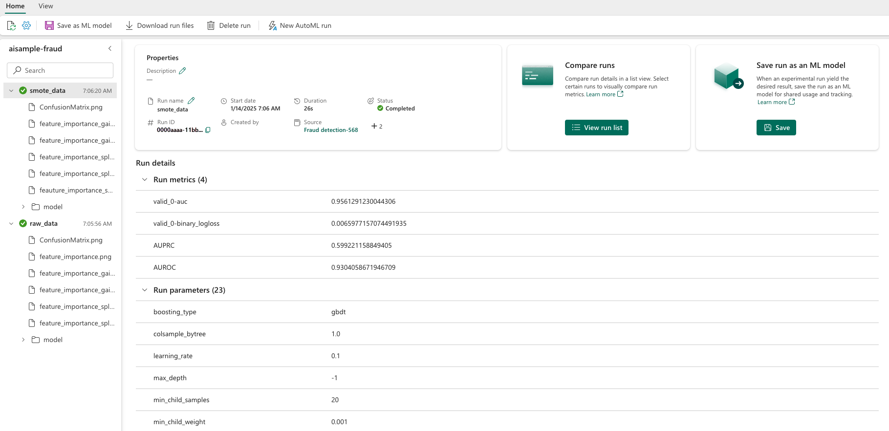
如下图所示,系统会记录每个试验及其各自的名称。 可以在工作区中跟踪试验参数和性能指标。
下图显示了在均衡数据集上训练的模型的性能指标( 在版本 2 中):
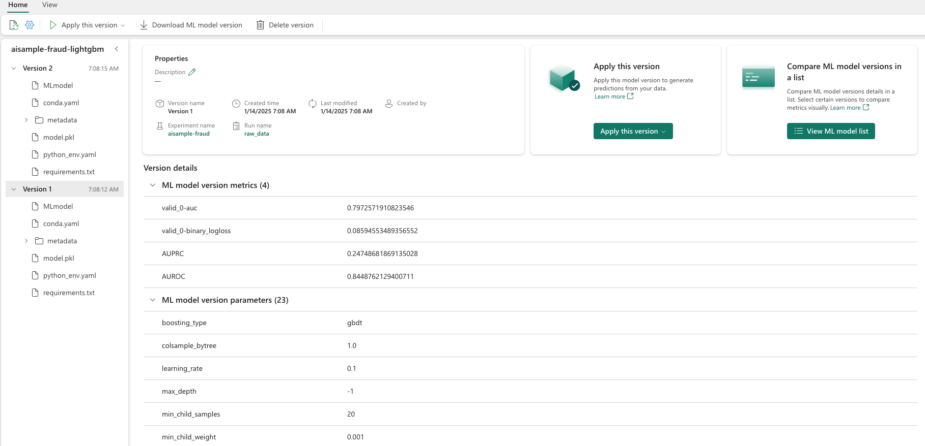
选择 版本 1 以查看在不平衡数据集上训练的模型的指标。 比较指标时,会看到使用均衡数据集训练的模型的 AUROC 更高。 这些结果表明,此模型更好地正确预测 0 类作为 0,并将 1 类预测为 1。
步骤 5:注册模型
使用 MLflow 注册两个模型:
# Register the model
registered_model_name = f"{EXPERIMENT_NAME}-lightgbm"

raw_model_uri = "runs:/{}/model".format(raw_run.info.run_id)
mlflow.register_model(raw_model_uri, registered_model_name)

smote_model_uri = "runs:/{}/model".format(smote_run.info.run_id)
mlflow.register_model(smote_model_uri, registered_model_name)
步骤 6:保存预测结果
Microsoft Fabric用户可以使用 PREDICT 可缩放函数操作机器学习模型。 此函数支持任何计算引擎中的批处理评分(或批处理推理)。
可以直接从Microsoft Fabric笔记本或模型的项页生成批量预测。 有关 PREDICT 的详细信息,请参阅 在 Microsoft Fabric 中使用 PREDICT 进行模型评分。
加载性能更好的模型(版本 2)进行批量评分,并生成预测结果:
from synapse.ml.predict import MLFlowTransformer

spark.conf.set("spark.synapse.ml.predict.enabled", "true")

model = MLFlowTransformer(
    inputCols=feature_cols,
    outputCol="prediction",
    modelName=f"{EXPERIMENT_NAME}-lightgbm",
    modelVersion=2,
)

test_spark = spark.createDataFrame(data=test, schema=test.columns.to_list())

batch_predictions = model.transform(test_spark)
将预测结果保存到湖屋中:
# Save the predictions to the lakehouse
batch_predictions.write.format("delta").mode("overwrite").save(f"{DATA_FOLDER}/predictions/batch_predictions")