教程：使用 R 创建、评估和评分欺诈检测模型

本教程演示了 Microsoft Fabric 中 Synapse 数据科学工作流的端到端示例。 在此方案中，我们在 R 中生成欺诈检测模型，并使用基于历史数据训练的机器学习算法。 然后，我们使用模型来检测未来的欺诈交易。

本教程介绍以下步骤：

• 安装自定义库
• 加载数据
• 通过探索性数据分析了解和处理数据，并显示 Fabric Data Wrangler 功能的用法
• 使用 LightGBM 训练机器学习模型
• 使用机器学习模型进行评分和预测

先决条件

• 获取 Microsoft Fabric 订阅。 或者，注册免费的 Microsoft Fabric 试用版。

• 登录 Microsoft Fabric。

• 使用主页左下侧的体验切换器切换到 Fabric。

  

• 如有必要，请创建 Microsoft Fabric 湖屋，如在 Microsoft Fabric 中创建湖屋中所述。

在笔记本中继续操作

可以选择以下选项之一以在笔记中继续操作：

• 在 Synapse Data Science 体验中打开并运行内置笔记本
• 将笔记本从 GitHub 上传到 Synapse 数据科学体验

打开内置笔记本

本教程随附欺诈检测示例笔记本。

1. 若要打开本教程的示例笔记本，请按照 为数据科学教程准备系统中的说明进行操作。

2. 在开始运行代码之前，请务必将湖屋附加到笔记本。

从 GitHub 导入笔记本

本教程随附 AIsample - R Fraud Detection.ipynb 笔记本。

• 若要打开本教程随附的笔记本，请按照 为数据科学教程准备系统 中的说明将笔记本导入工作区。

• 如果要复制并粘贴此页面中的代码，可以 创建新的笔记本。

• 在开始运行代码之前，请务必将湖屋附加到笔记本。

步骤 1：安装自定义库

对于机器学习模型开发或即席数据分析，可能需要为 Apache Spark 会话快速安装自定义库。 有两个选项可用于安装库。

• 请使用内联安装资源（例如 install.packages 和 devtools::install_version）进行安装，仅限于当前笔记本。
• 或者，可以创建 Fabric 环境、从公共源安装库或将自定义库上传到该环境，然后工作区管理员可以将环境附加为工作区的默认值。 然后，环境中的所有库将可用于工作区中的任何笔记本和 Spark 任务定义。 有关环境的详细信息，请参阅 在 Microsoft Fabric中创建、配置和使用环境。

在本教程中，使用 install.version() 安装不平衡学习库：

# Install dependencies
devtools::install_version("bnlearn", version = "4.8")
# Install imbalance for SMOTE
devtools::install_version("imbalance", version = "1.0.2.1")

步骤 2：加载数据

欺诈检测数据集包含 2013 年 9 月的信用卡交易，欧洲持卡人在两天内进行的信用卡交易。 由于应用于原始特征的主体组件分析（PCA）转换，数据集仅包含数值特征。 PCA 转换了除 Time 和 Amount以外的所有功能。 为了保护机密性，我们无法提供有关数据集的原始功能或更多背景信息。

这些详细信息描述了数据集：

• V1、V2、V3...、V28 功能是使用 PCA 获取的主要组件
• Time 特性包含一次交易与数据集中第一次交易之间所经过的秒数
• Amount 特征是交易金额。 可以使用此功能进行依赖于示例的成本敏感型学习
• Class 列是响应（目标）变量。 欺诈时其值为 1，否则为 0

在总计284,807笔交易中，只有492笔交易是欺诈性的。 该数据集高度不平衡，因为少数（欺诈）类仅占数据的约 0.172%。

下表显示了 creditcard.csv 数据的预览：

时间	V1	V2	V3	V4	V5	V6	V7	V8	V9	V10	V11	V12	V13	V14	V15	V16	V17	V18	V19	V20	V21	V22	V23	V24	V25	V26	V27	V28	金额	类
0	-1.3598071336738	-0.0727811733098497	2.53634673796914	1.37815522427443	-0.338320769942518	0.462387777762292	0.239598554061257	0.0986979012610507	0.363786969611213	0.0907941719789316	-0.551599533260813	-0.617800855762348	-0.991389847235408	-0.311169353699879	1.46817697209427	-0.470400525259478	0.207971241929242	0.0257905801985591	0.403992960255733	0.251412098239705	-0.018306777944153	0.277837575558899	-0.110473910188767	0.0669280749146731	0.128539358273528	-0.189114843888824	0.133558376740387	-0.0210530534538215	149.62	"0"
0	1.19185711131486	0.26615071205963	0.16648011335321	0.448154078460911	0.0600176492822243	-0.0823608088155687	-0.0788029833323113	0.0851016549148104	-0.255425128109186	-0.166974414004614	1.61272666105479	1.06523531137287	0.48909501589608	-0.143772296441519	0.635558093258208	0.463917041022171	-0.114804663102346	-0.183361270123994	-0.145783041325259	-0.0690831352230203	-0.225775248033138	-0.638671952771851	0.101288021253234	-0.339846475529127	0.167170404418143	0.125894532368176	-0.00898309914322813	0.0147241691924927	2.69	"0"

下载数据集并上传到湖屋

定义这些参数，以便可以将此笔记本用于不同的数据集：

IS_CUSTOM_DATA <- FALSE  # If TRUE, the dataset has to be uploaded manually

IS_SAMPLE <- FALSE  # If TRUE, use only rows of data for training; otherwise, use all data
SAMPLE_ROWS <- 5000  # If IS_SAMPLE is True, use only this number of rows for training

DATA_ROOT <- "/lakehouse/default"
DATA_FOLDER <- "Files/fraud-detection"  # Folder with data files
DATA_FILE <- "creditcard.csv"  # Data file name

此代码下载数据集的公开可用版本，然后将其存储在 Fabric Lakehouse 中。

重要

在运行笔记本之前，请务必向笔记本添加湖屋。 否则，将遇到错误。

if (!IS_CUSTOM_DATA) {
    # Download data files into a lakehouse if they don't exist
    library(httr)
    
    remote_url <- "https://synapseaisolutionsa.blob.core.windows.net/public/Credit_Card_Fraud_Detection"
    fname <- "creditcard.csv"
    download_path <- file.path(DATA_ROOT, DATA_FOLDER, "raw")

    dir.create(download_path, showWarnings = FALSE, recursive = TRUE)
    if (!file.exists(file.path(download_path, fname))) {
        r <- GET(file.path(remote_url, fname), timeout(30))
        writeBin(content(r, "raw"), file.path(download_path, fname))
    }
    message("Downloaded demo data files into lakehouse.")
}

从湖屋中读取原始日期数据

此代码从湖屋的“文件”一节读取原始数据：

data_df <- read.csv(file.path(DATA_ROOT, DATA_FOLDER, "raw", DATA_FILE))

步骤 3：执行探索性数据分析

使用 display 命令查看数据集的高级统计信息：

display(as.DataFrame(data_df, numPartitions = 3L))

# Print dataset basic information
message(sprintf("records read: %d", nrow(data_df)))
message("Schema:")
str(data_df)

# If IS_SAMPLE is True, use only SAMPLE_ROWS of rows for training
if (IS_SAMPLE) {
    data_df = sample_n(data_df, SAMPLE_ROWS)
}

打印数据集中类的分布：

# The distribution of classes in the dataset
message(sprintf("No Frauds %.2f%% of the dataset\n", round(sum(data_df$Class == 0)/nrow(data_df) * 100, 2)))
message(sprintf("Frauds %.2f%% of the dataset\n", round(sum(data_df$Class == 1)/nrow(data_df) * 100, 2)))

此类分布表明，大多数交易都是非欺诈的。 因此，在模型定型之前需要数据预处理，以避免过度拟合。

查看欺诈交易与非欺诈交易的分布情况

通过图表查看欺诈交易与非欺诈交易的分布，以展示数据集中的类别不平衡：

library(ggplot2)

ggplot(data_df, aes(x = factor(Class), fill = factor(Class))) +
  geom_bar(stat = "count") +
  scale_x_discrete(labels = c("no fraud", "fraud")) +
  ggtitle("Class Distributions \n (0: No Fraud || 1: Fraud)") +
  theme(plot.title = element_text(size = 10))

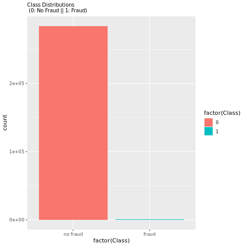
绘图清楚地显示了数据集不平衡：

显示五数字摘要

使用箱形图显示交易金额的五数字摘要（最小值、第一四分位数、中位数、第三四分位数和最大值）：

library(ggplot2)
library(dplyr)

ggplot(data_df, aes(x = as.factor(Class), y = Amount, fill = as.factor(Class))) +
  geom_boxplot(outlier.shape = NA) +
  scale_x_discrete(labels = c("no fraud", "fraud")) +
  ggtitle("Boxplot without Outliers") +
  coord_cartesian(ylim = quantile(data_df$Amount, c(0.05, 0.95)))

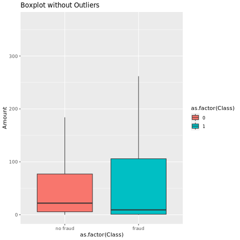
对于高度不平衡的数据，框图可能不会显示准确的见解。 但是，可以先解决 Class 不平衡问题，然后创建相同的绘图，以获取更准确的见解。

步骤 4：训练和评估模型

在这里，你将训练 LightGBM 模型来对欺诈交易进行分类。 在不平衡数据集和均衡数据集上训练 LightGBM 模型。 然后，比较这两个模型的性能。

准备训练和测试数据集

在训练之前，将数据拆分为训练数据集和测试数据集：

# Split the dataset into training and test datasets
set.seed(42)
train_sample_ids <- base::sample(seq_len(nrow(data_df)), size = floor(0.85 * nrow(data_df)))

train_df <- data_df[train_sample_ids, ]
test_df <- data_df[-train_sample_ids, ]

将 SMOTE 应用于训练数据集

不平衡的分类有问题。 对于模型来说，它太少了少数类示例，无法有效地了解决策边界。 合成少数类过度采样技术 (SMOTE) 可以解决此问题。 SMOTE 是合成少数民族类新样本的最广泛使用的方法。 可以使用在步骤 1 中安装的 imbalance 库访问 SMOTE。

仅将 SMOTE 应用于训练数据集，而不是测试数据集。 使用测试数据对模型进行评分时，您需要对模型在未见生产数据上的性能进行一个近似评估。 对于有效的近似值，测试数据依赖于原始不平衡分布来尽可能接近生产数据。

# Apply SMOTE to the training dataset
library(imbalance)

# Print the shape of the original (imbalanced) training dataset
train_y_categ <- train_df %>% select(Class) %>% table
message(
    paste0(
        "Original dataset shape ",
        paste(names(train_y_categ), train_y_categ, sep = ": ", collapse = ", ")
    )
)

# Resample the training dataset by using SMOTE
smote_train_df <- train_df %>%
    mutate(Class = factor(Class)) %>%
    oversample(ratio = 0.99, method = "SMOTE", classAttr = "Class") %>%
    mutate(Class = as.integer(as.character(Class)))

# Print the shape of the resampled (balanced) training dataset
smote_train_y_categ <- smote_train_df %>% select(Class) %>% table
message(
    paste0(
        "Resampled dataset shape ",
        paste(names(smote_train_y_categ), smote_train_y_categ, sep = ": ", collapse = ", ")
    )
)

有关 SMOTE 的详细信息，请参阅 CRAN 网站上的“imbalance”包和处理不均衡数据集资源。

使用 LightGBM 训练模型

使用不平衡数据集和通过 SMOTE 处理后的均衡数据集来训练 LightGBM 模型。 然后，比较其性能：

# Train LightGBM for both imbalanced and balanced datasets and define the evaluation metrics
library(lightgbm)

# Get the ID of the label column
label_col <- which(names(train_df) == "Class")

# Convert the test dataset for the model
test_mtx <- as.matrix(test_df)
test_x <- test_mtx[, -label_col]
test_y <- test_mtx[, label_col]

# Set up the parameters for training
params <- list(
    objective = "binary",
    learning_rate = 0.05,
    first_metric_only = TRUE
)

# Train for the imbalanced dataset
message("Start training with imbalanced data:")
train_mtx <- as.matrix(train_df)
train_x <- train_mtx[, -label_col]
train_y <- train_mtx[, label_col]
train_data <- lgb.Dataset(train_x, label = train_y)
valid_data <- lgb.Dataset.create.valid(train_data, test_x, label = test_y)
model <- lgb.train(
    data = train_data,
    params = params,
    eval = list("binary_logloss", "auc"),
    valids = list(valid = valid_data),
    nrounds = 300L
)

# Train for the balanced (via SMOTE) dataset   
message("\n\nStart training with balanced data:")
smote_train_mtx <- as.matrix(smote_train_df)
smote_train_x <- smote_train_mtx[, -label_col]
smote_train_y <- smote_train_mtx[, label_col]
smote_train_data <- lgb.Dataset(smote_train_x, label = smote_train_y)
smote_valid_data <- lgb.Dataset.create.valid(smote_train_data, test_x, label = test_y)
smote_model <- lgb.train(
    data = smote_train_data,
    params = params,
    eval = list("binary_logloss", "auc"),
    valids = list(valid = smote_valid_data),
    nrounds = 300L
)

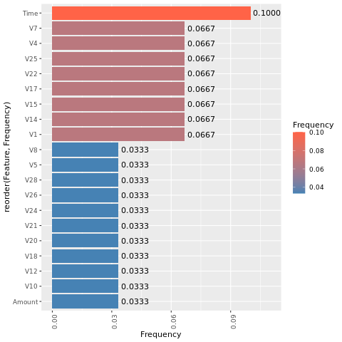
确定特征重要性

确定在不平衡数据集上训练的模型的特征重要性：

imp <- lgb.importance(model, percentage = TRUE)
ggplot(imp, aes(x = Frequency, y = reorder(Feature, Frequency), fill = Frequency)) +
  scale_fill_gradient(low="steelblue", high="tomato") +
  geom_bar(stat = "identity") +
  geom_text(aes(label = sprintf("%.4f", Frequency)), hjust = -0.1) +
  theme(axis.text.x = element_text(angle = 90)) +
  xlim(0, max(imp$Frequency) * 1.1)

对于在均衡（通过 SMOTE）数据集上训练的模型，请计算特征重要性：

smote_imp <- lgb.importance(smote_model, percentage = TRUE)
ggplot(smote_imp, aes(x = Frequency, y = reorder(Feature, Frequency), fill = Frequency)) +
  geom_bar(stat = "identity") +
  scale_fill_gradient(low="steelblue", high="tomato") +
  geom_text(aes(label = sprintf("%.4f", Frequency)), hjust = -0.1) +
  theme(axis.text.x = element_text(angle = 90)) +
  xlim(0, max(smote_imp$Frequency) * 1.1)

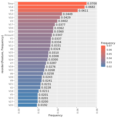
这些绘图的比较清楚地表明，均衡和不平衡的训练数据集具有很大的特征重要性差异。

评估模型

在这里，你将评估两个已训练的模型：

• model，使用原始且不均衡的数据进行训练
• smote_model，使用均衡数据进行训练

preds <- predict(model, test_mtx[, -label_col])
smote_preds <- predict(smote_model, test_mtx[, -label_col])

使用混淆矩阵评估模型性能

混淆矩阵显示以下内容的数量：

• 真正 (TP)
• 真负 (TN)
• 假正 (FP)
• 假负 (FP)

此数量是模型在使用测试数据进行评分时产生的。 对于二元分类，模型返回 2x2 混淆矩阵。 对于多类分类，模型返回 nxn 混淆矩阵，其中 n 是类数。

1. 使用混淆矩阵汇总训练的机器学习模型对测试数据的性能：

   plot_cm <- function(preds, refs, title) {
       library(caret)
       cm <- confusionMatrix(factor(refs), factor(preds))
       cm_table <- as.data.frame(cm$table)
       cm_table$Prediction <- factor(cm_table$Prediction, levels=rev(levels(cm_table$Prediction)))
   
       ggplot(cm_table, aes(Reference, Prediction, fill = Freq)) +
               geom_tile() +
               geom_text(aes(label = Freq)) +
               scale_fill_gradient(low = "white", high = "steelblue", trans = "log") +
               labs(x = "Prediction", y = "Reference", title = title) +
               scale_x_discrete(labels=c("0", "1")) +
               scale_y_discrete(labels=c("1", "0")) +
               coord_equal() +
               theme(legend.position = "none")
   }
   

2. 绘制在不平衡数据集上训练的模型的混淆矩阵：

   # The value of the prediction indicates the probability that a transaction is fraud
   # Use 0.5 as the threshold for fraud/no-fraud transactions
   plot_cm(ifelse(preds > 0.5, 1, 0), test_df$Class, "Confusion Matrix (Imbalanced dataset)")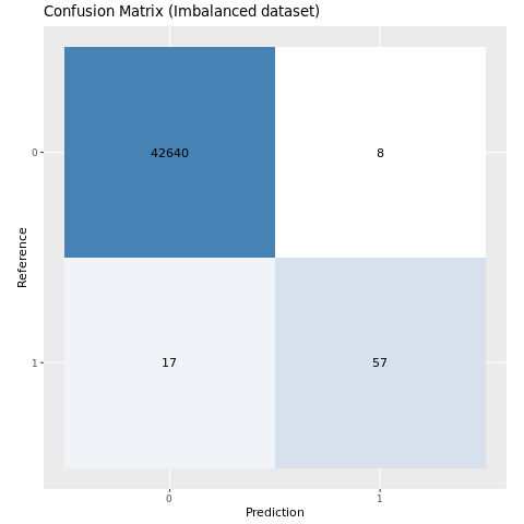
   

   

3. 绘制在均衡数据集上训练的模型的混淆矩阵：

   plot_cm(ifelse(smote_preds > 0.5, 1, 0), test_df$Class, "Confusion Matrix (Balanced dataset)")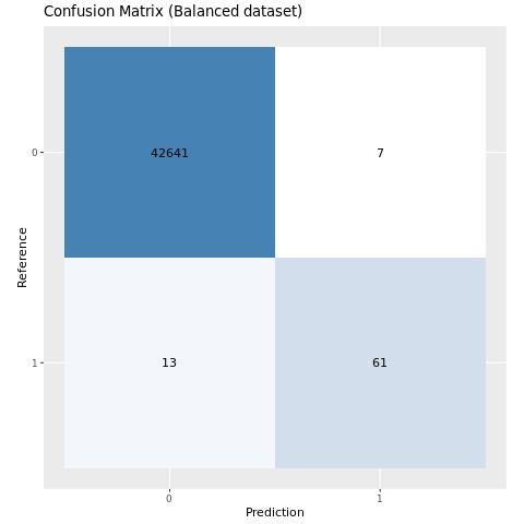
   

   

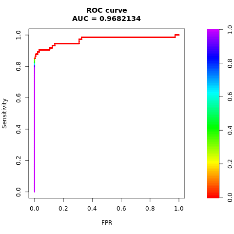
使用 AUC-ROC 和 AUPRC 度量值评估模型性能

接收器操作特征曲线（AUC-ROC）下的面积用于评估二元分类器的性能。 AUC-ROC 图表可视化展示真正阳性率（TPR）与假阳性率（FPR）之间的关系。

在某些情况下，根据“精准率-召回率曲线下面积 (AUPRC)”度量值来评估分类器更为合适。 AUPRC 曲线合并了以下速率：

• 精度或正预测值（PPV）
• 召回率或 TPR

# Use the PRROC package to help calculate and plot AUC-ROC and AUPRC
install.packages("PRROC", quiet = TRUE)
library(PRROC)

计算 AUC-ROC 和 AUPRC 指标

计算并绘制两个模型的 AUC-ROC 和 AUPRC 指标。

不平衡数据集

计算预测：

fg <- preds[test_df$Class == 1]
bg <- preds[test_df$Class == 0]

打印 AUC-ROC 曲线下的面积：

# Compute AUC-ROC
roc <- roc.curve(scores.class0 = fg, scores.class1 = bg, curve = TRUE)
print(roc)

绘制 AUC-ROC 曲线：

# Plot AUC-ROC
plot(roc)

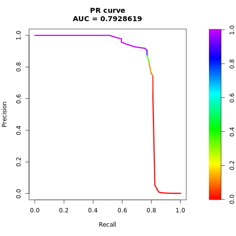
打印 AUPRC 曲线：

# Compute AUPRC
pr <- pr.curve(scores.class0 = fg, scores.class1 = bg, curve = TRUE)
print(pr)

绘制 AUPRC 曲线：

# Plot AUPRC
plot(pr)

均衡（通过 SMOTE）数据集

计算预测：

smote_fg <- smote_preds[test_df$Class == 1]
smote_bg <- smote_preds[test_df$Class == 0]

打印 AUC-ROC 曲线：

# Compute AUC-ROC
smote_roc <- roc.curve(scores.class0 = smote_fg, scores.class1 = smote_bg, curve = TRUE)
print(smote_roc)

绘制 AUC-ROC 曲线：

# Plot AUC-ROC
plot(smote_roc)

打印 AUPRC 曲线：

# Compute AUPRC
smote_pr <- pr.curve(scores.class0 = smote_fg, scores.class1 = smote_bg, curve = TRUE)
print(smote_pr)

绘制 AUPRC 曲线：

# Plot AUPRC
plot(smote_pr)

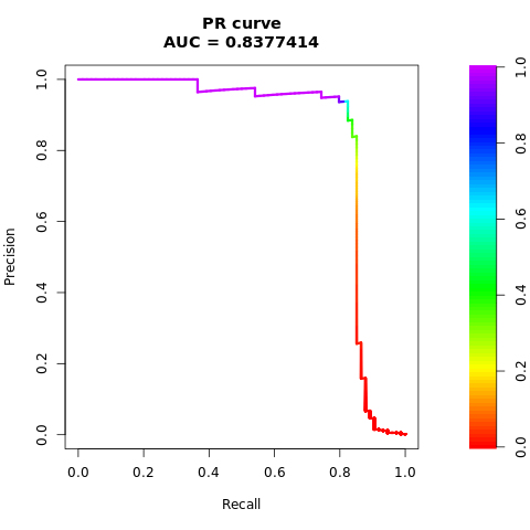
先前的数据清楚地表明，在均衡数据集上训练的模型在AUC-ROC和AUPRC分数上均优于在不平衡数据集上训练的模型。 此结果表明，在处理高度不平衡的数据时，SMOTE 可有效地提高模型性能。

相关内容

• Microsoft Fabric 中的 机器学习模型
• 训练机器学习模型
• Microsoft Fabric 中的机器学习试验