本教程演示了 Microsoft Fabric 中 Synapse 数据科学工作流的端到端示例。 此方案生成一个预测模型,该模型使用历史销售数据来预测超级商店的产品类别销售额。
预测是销售中的关键资产。 它结合了历史数据和预测方法,提供有关未来趋势的见解。 预测可以分析过去的销售额,以确定模式。 它还可以从消费者行为中学习,以优化库存、生产和营销策略。 这种主动方法可增强动态市场中的适应性、响应能力和整体业务性能。
本教程介绍以下步骤:
- 加载数据
- 使用探索性数据分析来了解和处理数据
- 使用开源软件包训练机器学习模型
- 使用 MLflow 和 Fabric 的自动记录功能来跟踪试验
- 保存最终的机器学习模型并进行预测
- 使用 Power BI 可视化效果显示模型性能
先决条件
获取 Microsoft Fabric 订阅。 或者,注册免费的 Microsoft Fabric 试用版。
登录 Microsoft Fabric。
使用主页左下侧的体验切换器切换到 Fabric。
- 如有必要,请按照 在 Microsoft Fabric 中创建 lakehouse 资源中的描述创建 Microsoft Fabric 湖仓。
在笔记本中继续操作
若要在笔记本中跟随学习,您有以下选项可供选择:
- 在 Synapse Data Science 体验中打开并运行内置笔记本
- 将笔记本从 GitHub 上传到 Synapse 数据科学体验
打开内置笔记本
本教程随附示例“销售预测”笔记本。
若要打开本教程的示例笔记本,请按照 为数据科学教程准备系统中的说明进行操作。
在开始运行代码之前,请务必将湖屋附加到笔记本。
从 GitHub 导入笔记本
本教程随附 AIsample - Superstore Forecast.ipynb 笔记本。
若要打开本教程随附的笔记本,请按照 为数据科学教程准备系统 中的说明将笔记本导入工作区。
如果要复制并粘贴此页面中的代码,可以 创建新的笔记本。
在开始运行代码之前,请务必将湖屋连接到笔记本。
步骤 1:加载数据
数据集有 9,995 个各种产品的销售额实例。 它还包括 21 个属性。 笔记本使用名为 Superstore.xlsx的文件。 该文件具有此表结构:
| 行 ID | 订单 ID | 订单日期 | 发货日期 | 发货模式 | 客户 ID | 客户名称 | 客户细分 | 国家 | 城市 | 州 | 邮政编码 | 区域 | 产品 ID | 类别 | 子类别 | 产品名称 | Sales | 数量 | 折扣 | 利润 |
|---|---|---|---|---|---|---|---|---|---|---|---|---|---|---|---|---|---|---|---|---|
| 4 | US-2015-108966 | 2015-10-11 | 2015-10-18 | 标准类 | SO-20335 | Sean O'Donnell | 消费者 | 美国 | 劳德代尔堡 | 佛罗里达州 | 33311 | 南 | FUR-TA-10000577 | 家具 | 表 | 布雷特福德 CR4500 系列纤细矩形桌子 | 957.5775 | 5 | 0.45 | -383.0310 |
| 11 | CA-2014-115812 | 2014-06-09 | 2014-06-09 | 标准类 | 标准类 | 布罗西娜·霍夫曼 | 消费者 | 美国 | 洛杉矶 | 加州 | 90032 | 西部 | FUR-TA-10001539 | 家具 | 表 | Chromcraft 矩形会议桌 | 1706.184 | 9 | 0.2 | 85.3092 |
| 31 | US-2015-150630 | 2015-09-17 | 2015-09-21 | 标准类 | TB-21520 | 特蕾西·布卢姆斯坦 | 消费者 | 美国 | 费城 | 宾夕法尼亚州 | 19140 | 东部 | OFF-EN-10001509 | Office 用品 | 信封 | 聚丙烯绳扣信封 | 3.264 | 2 | 0.2 | 1.1016 |
以下代码片段定义了特定参数,以便可以将此笔记本用于不同的数据集:
IS_CUSTOM_DATA = False  # If TRUE, the dataset has to be uploaded manually

IS_SAMPLE = False  # If TRUE, use only rows of data for training; otherwise, use all data
SAMPLE_ROWS = 5000  # If IS_SAMPLE is True, use only this number of rows for training

DATA_ROOT = "/lakehouse/default"
DATA_FOLDER = "Files/salesforecast"  # Folder with data files
DATA_FILE = "Superstore.xlsx"  # Data file name

EXPERIMENT_NAME = "aisample-superstore-forecast"  # MLflow experiment name
下载数据集并上传到湖仓 (Lakehouse)
以下代码片段下载公开可用的数据集版本,然后将该数据集存储在 Fabric Lakehouse 中:
重要
在运行笔记本之前,您必须 添加 Lakehouse 到笔记本。 否则,会发生错误。
import os, requests
if not IS_CUSTOM_DATA:
    # Download data files into the lakehouse if they're not already there
    remote_url = "https://synapseaisolutionsa.z13.web.core.windows.net/data/Forecast_Superstore_Sales"
    file_list = ["Superstore.xlsx"]
    download_path = "/lakehouse/default/Files/salesforecast/raw"

    if not os.path.exists("/lakehouse/default"):
        raise FileNotFoundError(
            "Default lakehouse not found, please add a lakehouse and restart the session."
        )
    os.makedirs(download_path, exist_ok=True)
    for fname in file_list:
        if not os.path.exists(f"{download_path}/{fname}"):
            r = requests.get(f"{remote_url}/{fname}", timeout=30)
            with open(f"{download_path}/{fname}", "wb") as f:
                f.write(r.content)
    print("Downloaded demo data files into lakehouse.")
设置 MLflow 试验跟踪
Microsoft Fabric 会在训练机器学习模型时自动捕获输入参数值和输出指标。 这扩展了 MLflow 自动记录功能。 然后,信息将记录到工作区,你可以在其中使用 MLflow API 或工作区中的相应试验访问和可视化它。 有关自动记录的详细信息,请访问 Microsoft Fabric 资源中的自动记录 。
若要在笔记本会话中关闭 Microsoft Fabric 自动记录,请调用 mlflow.autolog() 并设置 disable=True,如以下代码片段所示:
# Set up MLflow for experiment tracking
import mlflow

mlflow.set_experiment(EXPERIMENT_NAME)
mlflow.autolog(disable=True)  # Turn off MLflow autologging
从湖仓中读取原始数据
以下代码片段从 Lakehouse 的 “文件” 部分读取原始数据。 它还为不同的日期部分添加更多列。 相同的信息将用来创建一个分区的增量表。 由于原始数据存储为 Excel 文件,因此必须使用 pandas 读取它。
import pandas as pd
df = pd.read_excel("/lakehouse/default/Files/salesforecast/raw/Superstore.xlsx")
步骤 2:执行探索性数据分析
导入库
在开始分析之前导入所需的库:
# Importing required libraries
import warnings
import itertools
import numpy as np
import matplotlib.pyplot as plt
warnings.filterwarnings("ignore")
plt.style.use('fivethirtyeight')
import pandas as pd
import statsmodels.api as sm
import matplotlib
matplotlib.rcParams['axes.labelsize'] = 14
matplotlib.rcParams['xtick.labelsize'] = 12
matplotlib.rcParams['ytick.labelsize'] = 12
matplotlib.rcParams['text.color'] = 'k'
from sklearn.metrics import mean_squared_error,mean_absolute_percentage_error
显示原始数据
若要更好地了解数据集本身,请手动查看数据的子集。 使用 display 函数打印数据帧。 视图 Chart 可以轻松可视化数据集的子集:
display(df)
本教程展示一个主要关注 Furniture 类别销售预测的笔记本。 此方法加快计算速度,并帮助显示模型的性能。 但是,此笔记本使用适应性强的技术。 可以扩展这些技术来预测其他产品类别的销售情况。 以下代码片段选择 Furniture 为产品类别:
# Select "Furniture" as the product category
furniture = df.loc[df['Category'] == 'Furniture']
print(furniture['Order Date'].min(), furniture['Order Date'].max())
预处理数据
实际业务方案通常需要以三个不同的类别预测销售额:
- 特定产品类别
- 特定客户类别
- 产品类别和客户类别的特定组合
以下代码片段删除不必要的列来预处理数据。 我们不需要某些列(Row ID、Order ID和Customer IDCustomer Name),因为它们没有相关性。 我们希望针对特定产品类别Furniture()预测整个州和区域的总体销售额。 因此,我们可以删除 State、 Region、 Country、 City和 Postal Code 列。 若要预测特定位置或类别的销售情况,可能需要相应地调整预处理步骤。
# Data preprocessing
cols = ['Row ID', 'Order ID', 'Ship Date', 'Ship Mode', 'Customer ID', 'Customer Name',
'Segment', 'Country', 'City', 'State', 'Postal Code', 'Region', 'Product ID', 'Category',
'Sub-Category', 'Product Name', 'Quantity', 'Discount', 'Profit']
# Drop unnecessary columns
furniture.drop(cols, axis=1, inplace=True)
furniture = furniture.sort_values('Order Date')
furniture.isnull().sum()
数据集每天进行结构化。 我们必须对 Order Date 列重新采样,因为我们希望开发模型来每月预测销售额。
首先,按 Furniture对 Order Date 类别进行分组。 接下来,计算每个组的 Sales 列的总和,以确定每个唯一的 Order Date 值的总销售额。 使用 Sales 频率对 MS 列进行重新采样,以实现按月聚合数据。 最后,计算每个月的平均销售值。 以下代码片段显示了以下步骤:
# Data preparation
furniture = furniture.groupby('Order Date')['Sales'].sum().reset_index()
furniture = furniture.set_index('Order Date')
furniture.index
y = furniture['Sales'].resample('MS').mean()
y = y.reset_index()
y['Order Date'] = pd.to_datetime(y['Order Date'])
y['Order Date'] = [i+pd.DateOffset(months=67) for i in y['Order Date']]
y = y.set_index(['Order Date'])
maximim_date = y.reset_index()['Order Date'].max()
在以下代码片段中,显示 Order Date 对 Sales 的影响,类别为 Furniture:
# Impact of order date on the sales
y.plot(figsize=(12, 3))
plt.show()
在进行任何统计分析之前,必须导入 statsmodels Python 模块。 此模块提供用于估计许多统计模型的类和函数。 它还提供用于进行统计测试和统计数据探索的类和函数。 以下代码片段显示了此步骤:
import statsmodels.api as sm
执行统计分析
时序以设置间隔跟踪这些数据元素,以确定时序模式中这些元素的变体:
级别:表示特定时间段的平均值的基本组件
趋势:描述时序是减少、保持不变还是随时间而增加
季节性:描述时序中的周期性信号,并查找影响时序模式增加或减少的循环事件
干扰/残差:指模型无法解释的时序数据中的随机波动和可变性。
以下代码片段在预处理后显示数据集的这些元素:
# Decompose the time series into its components by using statsmodels
result = sm.tsa.seasonal_decompose(y, model='additive')

# Labels and corresponding data for plotting
components = [('Seasonality', result.seasonal),
              ('Trend', result.trend),
              ('Residual', result.resid),
              ('Observed Data', y)]

# Create subplots in a grid
fig, axes = plt.subplots(nrows=4, ncols=1, figsize=(12, 7))
plt.subplots_adjust(hspace=0.8)  # Adjust vertical space
axes = axes.ravel()

# Plot the components
for ax, (label, data) in zip(axes, components):
    ax.plot(data, label=label, color='blue' if label != 'Observed Data' else 'purple')
    ax.set_xlabel('Time')
    ax.set_ylabel(label)
    ax.set_xlabel('Time', fontsize=10)
    ax.set_ylabel(label, fontsize=10)
    ax.legend(fontsize=10)

plt.show()
这些图描述了预测数据中的季节性、趋势和噪音。 可以捕获基础模式,并开发能够准确预测的模型,这些模型具有针对随机波动的复原能力。
步骤 3:训练和跟踪模型
有了可用的数据后,请定义预测模型。 在此笔记本中,应用季节性自动回归集成移动平均值(SARIMAX)预测模型,该模型包含外生因素。 SARIMAX 结合了自动回归(AR)和移动平均值(MA)组件、季节性差异和外部预测器,对时序数据进行准确灵活的预测。
还可以使用 MLflow 和 Fabric 自动记录来跟踪试验。 在此处,从湖屋加载增量表。 你可能会使用其他将湖屋视为源的增量表。 以下代码片段导入所需的库:
# Import required libraries for model evaluation
from sklearn.metrics import mean_squared_error, mean_absolute_percentage_error
优化超参数
SARIMAX 考虑到常规自动回归集成移动平均值(ARIMA)模式(p、、dq)中涉及的参数,并添加季节性参数(P、、D、Qs)。 这些 SARIMAX 模型参数分别称为order(p、d、q)和季节性差分(P、D、Q、s)。 因此,若要训练模型,必须先优化七个参数。
阶数参数:
p:AR 组件的顺序,表示用于预测当前值的时序中过去观测值的数目。通常,此参数应具有非负整数值。 常见值在
03范围内。 但是,根据特定的数据特征,可能会有较高的值。 较高的p值表示模型中过去值的内存更长。d:差异顺序,表示时序需要差异的次数才能实现固定性。此参数应具有非负整数值。 常见值在
02范围内。d的0值表示时序已经平稳。 较大的值表示使时间序列变得平稳所需的差分次数更高。q:MA 组件的阶数。 此参数表示用于预测当前值的过去白噪声误差词的数目。此参数应具有非负整数值。 常见值在
0到3的范围内,但某些时间序列可能需要更高的值。 较高的q值表示更依赖过去的误差词进行预测。
季节性顺序参数:
-
P:AR 组件的季节性顺序,类似于p参数,但涵盖季节性部分 -
D:差异的季节性顺序,类似于d参数,但涵盖季节性部分 -
Q:MA 组件的季节性顺序,类似于q参数,但涵盖季节性部分 -
s:每个季节性周期的时间步骤数(例如,对于具有每年季节性的每月数据,为 12 个)
# Hyperparameter tuning
p = d = q = range(0, 2)
pdq = list(itertools.product(p, d, q))
seasonal_pdq = [(x[0], x[1], x[2], 12) for x in list(itertools.product(p, d, q))]
print('Examples of parameter combinations for Seasonal ARIMA...')
print('SARIMAX: {} x {}'.format(pdq[1], seasonal_pdq[1]))
print('SARIMAX: {} x {}'.format(pdq[1], seasonal_pdq[2]))
print('SARIMAX: {} x {}'.format(pdq[2], seasonal_pdq[3]))
print('SARIMAX: {} x {}'.format(pdq[2], seasonal_pdq[4]))
SARIMAX 具有其他参数:
enforce_stationarity:在拟合 SARIMAX 模型之前,模型是否应对时序数据强制实施固定性。值
enforce_stationarityTrue(默认值)表示应由 SARIMAX 模型在时序数据上强制施加平稳性。 在拟合模型之前,SARIMAX 模型会自动对数据应用差分,使其平稳,如d和D阶数指定。 这是一种常见做法,因为许多时序模型(包括 SARIMAX)都假定固定数据。对于非平稳时间序列(例如,具有趋势或季节性特征的序列),最好设置
enforce_stationarityTrue,让 SARIMAX 模型处理差分以实现平稳性。 对于固定时序(例如,没有趋势或季节性的时序),请将enforce_stationarity设置为False以避免不必要的差异。enforce_invertibility:控制模型是否应在优化过程中对估计参数强制实施不可逆性。enforce_invertibility值True(默认值)表示 SARIMAX 模型应对估计参数强制实施不可逆性。 不可逆性可确保定义良好的模型,并且估计的 AR 和 MA 系数位于固定范围内。不可逆强制有助于确保 SARIMAX 模型符合稳定时序模型的理论要求。 它还有助于防止模型估计和稳定性问题。
模型 AR(1) 是默认值。 这指的是 (1, 0, 0)。 但是,常见的做法是尝试顺序参数和季节性顺序参数的不同组合,并评估数据集的模型性能。 相应的值可能因不同的时序而异。
确定最佳值通常涉及分析时序数据的自动更正函数(ACF)和部分自动更正函数(PACF)。 它还经常涉及使用模型选择条件 -例如,Akaike 信息条件(AIC)或贝伊西亚信息条件(BIC)。
优化超参数,如以下代码片段所示:
# Tune the hyperparameters to determine the best model
for param in pdq:
    for param_seasonal in seasonal_pdq:
        try:
            mod = sm.tsa.statespace.SARIMAX(y,
                                            order=param,
                                            seasonal_order=param_seasonal,
                                            enforce_stationarity=False,
                                            enforce_invertibility=False)
            results = mod.fit(disp=False)
            print('ARIMA{}x{}12 - AIC:{}'.format(param, param_seasonal, results.aic))
        except:
            continue
评估上述结果后,可以确定订单参数和季节性订单参数的值。 选择是 order=(0, 1, 1) 和 seasonal_order=(0, 1, 1, 12),它们具有最低的 AIC(例如 279.58)。 使用这些值来训练模型。 以下代码片段显示了此步骤:
训练模型
# Model training
mod = sm.tsa.statespace.SARIMAX(y,
                                order=(0, 1, 1),
                                seasonal_order=(0, 1, 1, 12),
                                enforce_stationarity=False,
                                enforce_invertibility=False)
results = mod.fit(disp=False)
print(results.summary().tables[1])
此代码可视化家具销售数据的时序预测。 绘制的结果显示了观测到的数据和一步向前预测,其中阴影区域表示置信区间。 以下代码片段显示了可视化效果:
# Plot the forecasting results
pred = results.get_prediction(start=maximim_date, end=maximim_date+pd.DateOffset(months=6), dynamic=False) # Forecast for the next 6 months (months=6)
pred_ci = pred.conf_int() # Extract the confidence intervals for the predictions
ax = y['2019':].plot(label='observed')
pred.predicted_mean.plot(ax=ax, label='One-step ahead forecast', alpha=.7, figsize=(12, 7))
ax.fill_between(pred_ci.index,
                pred_ci.iloc[:, 0],
                pred_ci.iloc[:, 1], color='k', alpha=.2)
ax.set_xlabel('Date')
ax.set_ylabel('Furniture Sales')
plt.legend()
plt.show()
# Validate the forecasted result
predictions = results.get_prediction(start=maximim_date-pd.DateOffset(months=6-1), dynamic=False)
# Forecast on the unseen future data
predictions_future = results.get_prediction(start=maximim_date+ pd.DateOffset(months=1),end=maximim_date+ pd.DateOffset(months=6),dynamic=False)
以下代码片段使用 predictions 它来评估模型的性能,方法是将其与实际值进行对比。
predictions_future 值指示未来的预测。
# Log the model and parameters
model_name = f"{EXPERIMENT_NAME}-Sarimax"
with mlflow.start_run(run_name="Sarimax") as run:
    mlflow.statsmodels.log_model(results,model_name,registered_model_name=model_name)
    mlflow.log_params({"order":(0,1,1),"seasonal_order":(0, 1, 1, 12),'enforce_stationarity':False,'enforce_invertibility':False})
    model_uri = f"runs:/{run.info.run_id}/{model_name}"
    print("Model saved in run %s" % run.info.run_id)
    print(f"Model URI: {model_uri}")
mlflow.end_run()
# Load the saved model
loaded_model = mlflow.statsmodels.load_model(model_uri)
步骤 4:为模型评分并保存预测
以下代码片段将实际值与预测值集成,以创建 Power BI 报表。 此外,它还将这些结果存储在数据湖仓中的表格中。
# Data preparation for Power BI visualization
Future = pd.DataFrame(predictions_future.predicted_mean).reset_index()
Future.columns = ['Date','Forecasted_Sales']
Future['Actual_Sales'] = np.NAN
Actual = pd.DataFrame(predictions.predicted_mean).reset_index()
Actual.columns = ['Date','Forecasted_Sales']
y_truth = y['2023-02-01':]
Actual['Actual_Sales'] = y_truth.values
final_data = pd.concat([Actual,Future])
# Calculate the mean absolute percentage error (MAPE) between 'Actual_Sales' and 'Forecasted_Sales'
final_data['MAPE'] = mean_absolute_percentage_error(Actual['Actual_Sales'], Actual['Forecasted_Sales']) * 100
final_data['Category'] = "Furniture"
final_data[final_data['Actual_Sales'].isnull()]
input_df = y.reset_index()
input_df.rename(columns = {'Order Date':'Date','Sales':'Actual_Sales'}, inplace=True)
input_df['Category'] = 'Furniture'
input_df['MAPE'] = np.NAN
input_df['Forecasted_Sales'] = np.NAN
# Write back the results into the lakehouse
final_data_2 = pd.concat([input_df,final_data[final_data['Actual_Sales'].isnull()]])
table_name = "Demand_Forecast_New_1"
spark.createDataFrame(final_data_2).write.mode("overwrite").format("delta").save(f"Tables/{table_name}")
print(f"Spark DataFrame saved to delta table: {table_name}")
步骤 5:在 Power BI 中可视化
Power BI 报表显示平均绝对百分比误差(MAPE)为 16.58。 MAPE 指标定义预测方法的准确性。 它表示预测数量与实际数量相比的准确性。
MAPE 是一个简单的指标。 10% MAPE 表示预测值与实际值之间的平均偏差是 10%,无论偏差是正还是负。 所需 MAPE 值的标准因行业而异。
此图中的浅蓝色线条表示实际销售值。 深蓝色线条表示预测的销售值。 实际销售额和预测销售额的比较显示,模型可有效预测 2023 年上半年 Furniture 类别的销售情况。
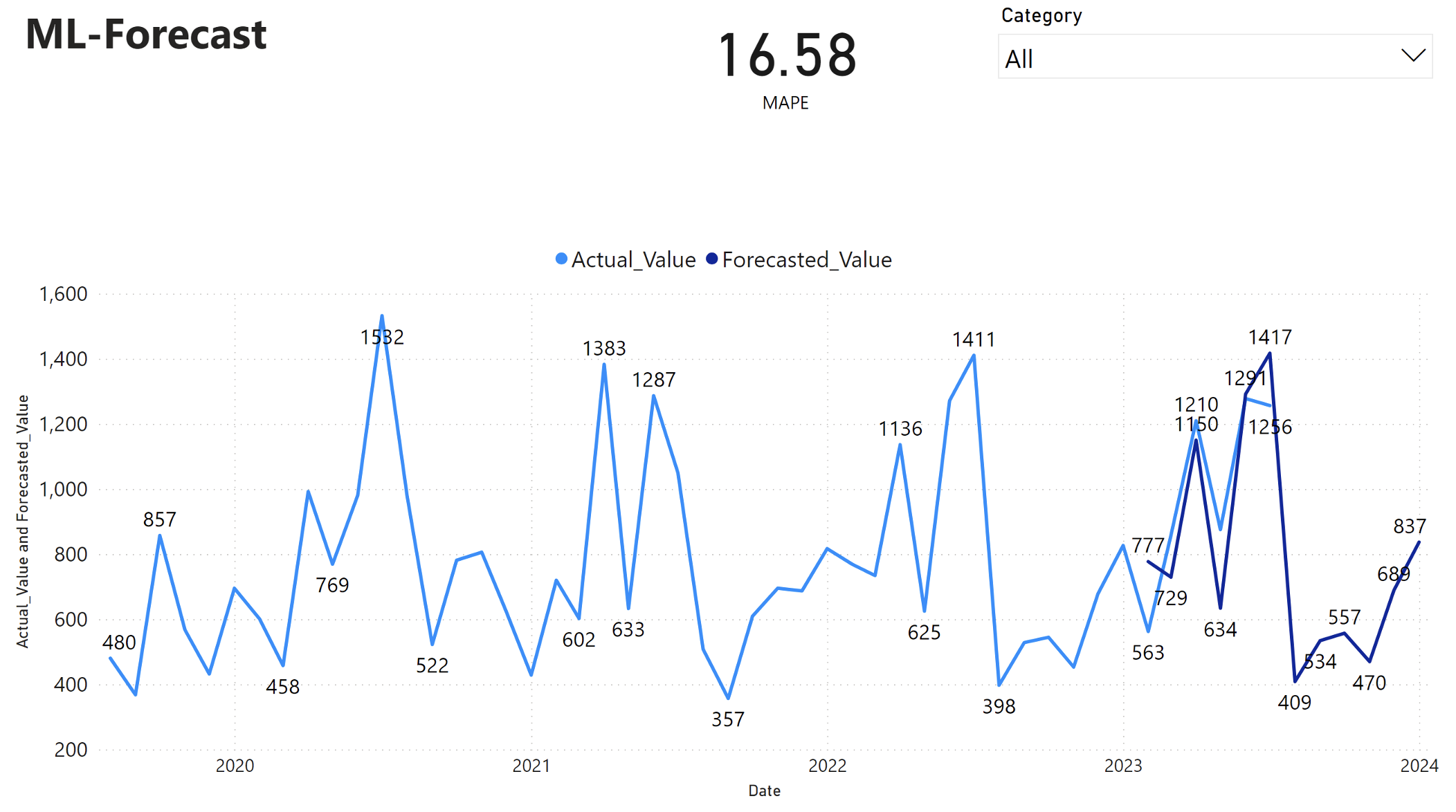
根据这一观察,我们可以有信心预测模型在 2023 年过去 6 个月的总销售额,并扩展到 2024 年。 这种信心可以告知有关库存管理、原材料采购和其他与业务相关的注意事项的战略决策。
相关内容
- 如何使用 Microsoft Fabric 笔记本
- Microsoft Fabric 中的 机器学习模型
- 训练机器学习模型
- Microsoft Fabric 中的机器学习试验