教學課程：建立、評估詐騙偵測模型及評分

本教學呈現資料科學工作流程的端到端範例。該情境透過訓練於歷史資料的機器學習演算法，建立詐欺偵測模型。隨後會使用模型，來偵測未來的詐騙交易。

本教學課程涵蓋了下列步驟：

安裝自訂程式庫
載入資料
使用探索式資料分析來了解和處理資料
使用 scikit-learn 訓練機器學習模型，並使用 MLflow 與 Fabric Autolog 功能追蹤實驗
儲存並註冊效能最高的machine learning模型
載入machine learning模型以進行評分與預測

必要條件

訂閱Microsoft Fabric。或者，註冊免費的Microsoft Fabric試用。
登入Microsoft Fabric。
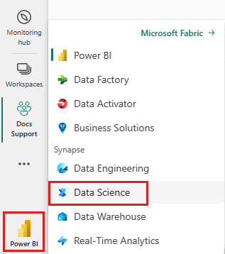
使用首頁左下角的體驗切換器切換到 Fabric。

如果有需要，請依照Create a lakehouse in Microsoft Fabric中所述，在 Microsoft Fabric 中建立湖屋。

遵循筆記本中的指示

要在筆記本中操作，請選取以下選項之一：

開啟並執行內建筆記本。
從 GitHub 上傳你的筆記本。

開啟內建筆記本

此教學課程隨附詐騙偵測筆記本範例。

若要開啟本教學課程的範例筆記本，請遵循中關於準備系統以進行數據科學教學課程的指示，。
開始執行程式碼之前，請務必將 lakehouse 連結至筆記本。

從 GitHub 匯入筆記本

本教學附有 AI範例 - Fraud Detection.ipynb 筆記本。

若要開啟本教學課程隨附的筆記本，請遵循準備系統以進行數據科學教學課程中的指示，將筆記本匯入工作區。
如果您想要複製並貼上此頁面中的程式碼，則可以建立新的筆記本。
開始執行程式碼之前，請務必將 Lakehouse 連結至筆記本。

步驟 1：安裝自訂程式庫

若用於機器學習模型開發或臨時資料分析，您可能需要快速安裝自訂程式庫以支援您的 Apache Spark 工作階段。安裝程式庫有兩個選項。

使用筆記本的內嵌安裝功能 (%pip 或 %conda)，僅在您目前的筆記本中安裝程式庫。
或者，你也可以建立 Fabric 環境，從公開來源安裝函式庫或上傳自訂函式庫，然後你的工作區管理員可以將該環境附加為工作區的預設。環境中的所有函式庫都可以在任何筆記本和工作區的 Spark 工作定義中使用。欲了解更多環境資訊，請參閱建立、配置及使用Microsoft Fabric中的環境。

在本教學課程中，使用 %pip install 在您的筆記本中安裝 imblearn 程式庫。

注意

執行 %pip install 之後，PySpark 核心會重新啟動。在執行任何其他資料格之前，請先安裝所需的程式庫。

# Use pip to install imblearn
%pip install imblearn

步驟 2：載入資料

詐騙偵測資料集包含2013年9月歐洲持卡人在兩天內進行的信用卡交易。由於套用至原始特徵的主體元件分析 (PCA) 轉換，資料集只包含數值特徵。 PCA 已轉換 Time 和 Amount 以外的所有特徵。為了保護機密性，原始特徵或更多資料集的背景資訊無法公開。

以下是描述資料集的詳細資料：

V1、V2、V3、...、V28這些特徵是利用 PCA 得到的主要成分。
特性 Time 包含交易與資料集中第一筆交易之間經過的秒數。
Amount 特徵為交易金額。你可以用這個功能來進行依賴範例且對成本敏感的學習。
Class 資料欄為回應 (目標) 變數。它的值在詐欺情況下是1，在其他情況下是0。

在總計 284,807 筆交易中，只有 492 筆交易具有詐騙性。資料集高度不平衡，因為少數 (詐騙) 類別只占資料的 0.172%。

下表顯示 creditcard.csv 資料的預覽：

時間	V1	V2	V3	V4	V5	V6	V7	V8	V9	V10	V11	V12	V13	V14	V15	V16	V17	V18	V19	V20	V21	V22	V23	V24	V25	V26	V27	V28	總數	類別
0	-1.3598071336738	-0.0727811733098497	2.53634673796914	1.37815522427443	-0.338320769942518	0.462387777762292	0.239598554061257	0.0986979012610507	0.363786969611213	0.0907941719789316	-0.551599533260813	-0.617800855762348	-0.991389847235408	-0.311169353699879	1.46817697209427	-0.470400525259478	0.207971241929242	0.0257905801985591	0.403992960255733	0.251412098239705	-0.018306777944153	0.277837575558899	-0.110473910188767	0.0669280749146731	0.128539358273528	-0.189114843888824	0.133558376740387	-0.0210530534538215	149.62	"0"
0	1.19185711131486	0.26615071205963	0.16648011335321	0.448154078460911	0.0600176492822243	-0.0823608088155687	-0.0788029833323113	0.0851016549148104	-0.255425128109186	-0.166974414004614	1.61272666105479	1.06523531137287	0.48909501589608	-0.143772296441519	0.635558093258208	0.463917041022171	-0.114804663102346	-0.183361270123994	-0.145783041325259	-0.0690831352230203	-0.225775248033138	-0.638671952771851	0.101288021253234	-0.339846475529127	0.167170404418143	0.125894532368176	-0.00898309914322813	0.0147241691924927	2.69	"0"

下載資料集並上傳至 Lakehouse

請定義這些參數，讓你能在不同資料集中使用這個筆記本：

IS_CUSTOM_DATA = False  # If True, the dataset has to be uploaded manually

TARGET_COL = "Class"  # Target column name
IS_SAMPLE = False  # If True, use only <SAMPLE_ROWS> rows of data for training; otherwise, use all data
SAMPLE_ROWS = 5000  # If IS_SAMPLE is True, use only this number of rows for training

DATA_FOLDER = "Files/fraud-detection/"  # Folder with data files
DATA_FILE = "creditcard.csv"  # Data file name

EXPERIMENT_NAME = "aisample-fraud"  # MLflow experiment name

此程式碼會下載公開版本的資料集，然後儲存在 Fabric 湖屋中。

重要

在運行筆記本之前，先加建一個湖邊小屋。否則就會發生錯誤。

if not IS_CUSTOM_DATA:
    # Download data files into the lakehouse if they're not already there
    import os, requests

    remote_url = "https://synapseaisolutionsa.z13.web.core.windows.net/data/Credit_Card_Fraud_Detection"
    fname = "creditcard.csv"
    download_path = f"/lakehouse/default/{DATA_FOLDER}/raw"

    if not os.path.exists("/lakehouse/default"):
        raise FileNotFoundError("Default lakehouse not found, please add a lakehouse and restart the session.")
    os.makedirs(download_path, exist_ok=True)
    if not os.path.exists(f"{download_path}/{fname}"):
        r = requests.get(f"{remote_url}/{fname}", timeout=30)
        with open(f"{download_path}/{fname}", "wb") as f:
            f.write(r.content)
    print("Downloaded demo data files into lakehouse.")

設定 MLflow 實驗追蹤

實驗追蹤程序會為您執行的每個實驗儲存所有相關實驗的相關資訊。有時候，做特定實驗無法獲得更好的結果。在這種情況下，停止實驗，嘗試新的。

資料科學包含自動記錄功能。此功能減少了在訓練過程中自動記錄machine learning模型參數、指標與項目所需的程式碼量。此功能可擴充 MLflow 自動記錄功能。它與資料科學工作負載有深度整合。

透過自動記錄，您可以輕鬆追蹤並比較不同模型與實驗的表現，無需手動追蹤。更多資訊，請參閱Microsoft Fabric 中的Autologging。

要在筆記本會話中停用Microsoft Fabric自動登入，請呼叫 mlflow.autolog() 並設定 disable=True：

# Set up MLflow for experiment tracking
import mlflow

mlflow.set_experiment(EXPERIMENT_NAME)
mlflow.autolog(disable=True)  # Disable MLflow autologging

從湖倉讀取原始數據

此程式碼會從 Lakehouse 讀取未經處理資料：

df = (
    spark.read.format("csv")
    .option("header", "true")
    .option("inferSchema", True)
    .load(f"{DATA_FOLDER}/raw/{DATA_FILE}")
    .cache()
)

步驟 3：執行探索式資料分析

在本節中，您會先探索未經處理資料和高階統計資料。然後，若要轉換資料，請將資料行轉換成正確的類型，並將其從 Spark DataFrame 轉換成 pandas DataFrame，以方便視覺化。最後，您會探索並視覺化資料中的類別分佈。

顯示未經處理資料

使用指令探索原始資料並查看高層統計數據 display 。欲了解更多關於資料視覺化的資訊，請參閱Microsoft Fabric 中的 Notebook 視覺化。
```
display(df)
```

列印資料集的一些基本資訊：

# Print dataset basic information
print("records read: " + str(df.count()))
print("Schema: ")
df.printSchema()

轉換資料

將資料集資料列轉換成正確的類型：

import pyspark.sql.functions as F

df_columns = df.columns
df_columns.remove(TARGET_COL)

# Ensure that TARGET_COL is the last column
df = df.select(df_columns + [TARGET_COL]).withColumn(TARGET_COL, F.col(TARGET_COL).cast("int"))

if IS_SAMPLE:
    df = df.limit(SAMPLE_ROWS)

將 Spark DataFrame 轉換成 pandas DataFrame，以方便視覺化和處理：
```
df_pd = df.toPandas()
```

探索資料集中的類別分佈

在資料集中顯示類別分佈：
```
# The distribution of classes in the dataset
print('No Frauds', round(df_pd['Class'].value_counts()[0]/len(df_pd) * 100,2), '% of the dataset')
print('Frauds', round(df_pd['Class'].value_counts()[1]/len(df_pd) * 100,2), '% of the dataset')
```
此程式碼會傳回此資料集類別分佈：99.83% No Frauds 和 0.17% Frauds。此類別分佈顯示大部分交易都是非詐騙性的。因此，在模型訓練前必須進行資料預處理，以避免過度擬合。

藉由檢視詐騙交易與非詐騙交易的分佈，使用繪圖來顯示資料集中的類別不平衡：

import seaborn as sns
import matplotlib.pyplot as plt

colors = ["#0101DF", "#DF0101"]
sns.countplot(x='Class', data=df_pd, palette=colors) 
plt.title('Class Distributions \n (0: No Fraud || 1: Fraud)', fontsize=10)

以盒狀圖顯示交易金額的五個數字摘要 (最小值、第一分位數、中位數、第三分位數和最大分數)：

fig, (ax1, ax2) = plt.subplots(ncols=2, figsize=(12,5))
s = sns.boxplot(ax = ax1, x="Class", y="Amount", hue="Class",data=df_pd, palette="PRGn", showfliers=True) # Remove outliers from the plot
s = sns.boxplot(ax = ax2, x="Class", y="Amount", hue="Class",data=df_pd, palette="PRGn", showfliers=False) # Keep outliers from the plot
plt.show()

針對高度不平衡的資料，盒狀圖可能不會顯示準確的深入解析。不過，您可以先解決 Class 不平衡問題，然後建立相同的繪圖，以取得更準確的深入解析。

步驟 4︰訓練及評估模型

在此步驟中，你訓練一個 LightGBM 模型來分類詐欺交易。您可同時在不平衡的資料集與平衡的資料集上訓練 LightGBM 模型。然後，比較這兩個模型的效能。

準備訓練和測試資料集

在定型之前，將資料分割為定型和測試資料集：

# Split the dataset into training and testing sets
from sklearn.model_selection import train_test_split

train, test = train_test_split(df_pd, test_size=0.15)
feature_cols = [c for c in df_pd.columns.tolist() if c not in [TARGET_COL]]

將 SMOTE 套用至訓練資料集

該 imblearn 程式庫使用綜合少數超取樣技術 (SMOTE) 方法來解決不平衡分類的問題。當少數類別的樣本不足時，可能會發生不平衡分類，這使得模型難以有效學習決策邊界。 SMOTE 是合成少數類別新樣本最廣泛使用的方法。

僅將 SMOTE 套用至訓練資料集，而不是測試資料集。當您使用測試資料為模型評分時，需要生產環境中未顯示資料上的近似模型效能。針對有效的近似值，您的測試資料倚賴原始不平衡分佈，以儘可能接近地呈現生產資料。

# Apply SMOTE to the training data
import pandas as pd
from collections import Counter
from imblearn.over_sampling import SMOTE

X = train[feature_cols]
y = train[TARGET_COL]
print("Original dataset shape %s" % Counter(y))

sm = SMOTE(random_state=42)
X_res, y_res = sm.fit_resample(X, y)
print("Resampled dataset shape %s" % Counter(y_res))

new_train = pd.concat([X_res, y_res], axis=1)

訓練machine learning模型並執行實驗

Microsoft Fabric 中的 Apache Spark 能利用大數據實現機器學習。透過使用 Apache Spark，你可以從大量結構化、非結構化及快速變化的資料中獲得寶貴的洞見。

在 Microsoft Fabric 中，有多種可用選項來訓練機器學習模型：Apache Spark MLlib、SynapseML 及其他開源函式庫。欲了解更多資訊，請參閱在 Microsoft Fabric 中訓練機器學習模型。

機器學習實驗作為所有相關機器學習運行的主要組織和控制單位。執行對應於模型程式碼的一次執行。 Machine learning experiment tracking 涉及管理所有實驗及其組成部分，例如參數、指標、模型及其他工件。

在實驗追蹤方面，你可以組織特定machine learning實驗的所有必要組成部分。此外，您可以使用已儲存的實驗輕鬆重現過去的結果。欲了解更多機器學習實驗資訊，請參閱機器學習實驗 in Microsoft Fabric。

若要追蹤更多計量、參數和檔案，請將 exclusive=False 設定為更新 MLflow 自動記錄組態：
```
mlflow.autolog(exclusive=False)
```

使用 LightGBM 訓練兩個模型。一個模型會處理不平衡的資料集，另一個模型會處理平衡資料集 (透過 SMOTE)。比較這兩個模型的效能。

import lightgbm as lgb

model = lgb.LGBMClassifier(objective="binary") # Imbalanced dataset
smote_model = lgb.LGBMClassifier(objective="binary") # Balanced dataset

# Train LightGBM for both imbalanced and balanced datasets and define the evaluation metrics
print("Start training with imbalanced data:\n")
with mlflow.start_run(run_name="raw_data") as raw_run:
    model = model.fit(
        train[feature_cols],
        train[TARGET_COL],
        eval_set=[(test[feature_cols], test[TARGET_COL])],
        eval_metric="auc",
        callbacks=[
            lgb.log_evaluation(10),
        ],
    )

print(f"\n\nStart training with balanced data:\n")
with mlflow.start_run(run_name="smote_data") as smote_run:
    smote_model = smote_model.fit(
        new_train[feature_cols],
        new_train[TARGET_COL],
        eval_set=[(test[feature_cols], test[TARGET_COL])],
        eval_metric="auc",
        callbacks=[
            lgb.log_evaluation(10),
        ],
    )

確定模型訓練的特徵重要性

針對您在不平衡資料集上訓練的模型，判斷特徵重要度：

with mlflow.start_run(run_id=raw_run.info.run_id):
    importance = lgb.plot_importance(
        model, title="Feature importance for imbalanced data"
    )
    importance.figure.savefig("feauture_importance.png")
    mlflow.log_figure(importance.figure, "feature_importance.png")

針對您在不平衡資料集上定型的模型，判斷特徵重要度。 SMOTE 產生平衡的資料：

with mlflow.start_run(run_id=smote_run.info.run_id):
    smote_importance = lgb.plot_importance(
        smote_model, title="Feature importance for balanced (via SMOTE) data"
    )
    smote_importance.figure.savefig("feauture_importance_smote.png")
    mlflow.log_figure(smote_importance.figure, "feauture_importance_smote.png")

當你用不平衡資料集訓練模型時，重要特徵與用平衡資料集訓練的模型有顯著差異。

評估模型

您會在此評估兩個訓練模型：

根據不平衡的原始資料訓練model
在平衡資料上對 smote_model 訓練

計算模型計量

定義一個 prediction_to_spark 函數，能進行預測並將預測結果轉換成 Spark DataFrame。接著你可以利用 SynapseML 計算預測結果的模型統計量。

from pyspark.sql.functions import col
from pyspark.sql.types import IntegerType, DoubleType

def prediction_to_spark(model, test):
    predictions = model.predict(test[feature_cols], num_iteration=model.best_iteration_)
    predictions = tuple(zip(test[TARGET_COL].tolist(), predictions.tolist()))
    dataColumns = [TARGET_COL, "prediction"]
    predictions = (
        spark.createDataFrame(data=predictions, schema=dataColumns)
        .withColumn(TARGET_COL, col(TARGET_COL).cast(IntegerType()))
        .withColumn("prediction", col("prediction").cast(DoubleType()))
    )

    return predictions

使用函 prediction_to_spark 數對兩個模型進行預測， model 且 smote_model：

predictions = prediction_to_spark(model, test)
smote_predictions = prediction_to_spark(smote_model, test)
predictions.limit(10).toPandas()

計算兩個模型的計量：

from synapse.ml.train import ComputeModelStatistics

metrics = ComputeModelStatistics(
    evaluationMetric="classification", labelCol=TARGET_COL, scoredLabelsCol="prediction"
).transform(predictions)

smote_metrics = ComputeModelStatistics(
    evaluationMetric="classification", labelCol=TARGET_COL, scoredLabelsCol="prediction"
).transform(smote_predictions)
display(metrics)

使用混淆矩陣評估模型效能

混淆矩陣會顯示數據的數量

真陽性 (TP)
真負類 (TN)
假陽性 (FP)
偽陰性 (FN)

這是模型使用測試資料進行評分後所產生的結果。針對二元分類，模型會傳回 2x2 混淆矩陣。針對多類別分類，模型會傳回 nxn 混淆矩陣，其中 n 為類別數目。

使用混淆矩陣來總結訓練好的machine learning模型在測試資料上的表現：

# Collect confusion matrix values
cm = metrics.select("confusion_matrix").collect()[0][0].toArray()
smote_cm = smote_metrics.select("confusion_matrix").collect()[0][0].toArray()
print(cm)

繪製經平衡數據訓練的 smote_model 預測之混淆矩陣：

# Plot the confusion matrix
import seaborn as sns

def plot(cm):
    """
    Plot the confusion matrix.
    """
    sns.set(rc={"figure.figsize": (5, 3.5)})
    ax = sns.heatmap(cm, annot=True, fmt=".20g")
    ax.set_title("Confusion Matrix")
    ax.set_xlabel("Predicted label")
    ax.set_ylabel("True label")
    return ax

with mlflow.start_run(run_id=smote_run.info.run_id):
    ax = plot(smote_cm)
    mlflow.log_figure(ax.figure, "ConfusionMatrix.png")

繪製 model 預測的混淆矩陣 (以原始、不平衡資料定型)：

with mlflow.start_run(run_id=raw_run.info.run_id):
    ax = plot(cm)
    mlflow.log_figure(ax.figure, "ConfusionMatrix.png")

使用 AUC-ROC 和 AUPRC 量值來評估模型效能

曲線下面積接收者操作特徵 (AUC-ROC) 量度評估二元分類器的效能。 AUC-ROC 圖表會視覺化確判率 (TPR) 與誤判率 (FPR) 之間的取捨。

在某些情況下，根據 Area Under the Precision-Recall Curve (AUPRC) 量值來評估分類器比較合適。 AUPRC 曲線會結合這些比率：

精確度或陽性預測值 (PPV)
召回率或真陽性率 (TPR)

要使用 AUC-ROC 和 AUPRC 量值來評估效能：

定義傳回 AUC-ROC 和 AUPRC 量值的函式：

from pyspark.ml.evaluation import BinaryClassificationEvaluator

def evaluate(predictions):
    """
    Evaluate the model by computing AUROC and AUPRC with the predictions.
    """

    # Initialize the binary evaluator
    evaluator = BinaryClassificationEvaluator(rawPredictionCol="prediction", labelCol=TARGET_COL)

    _evaluator = lambda metric: evaluator.setMetricName(metric).evaluate(predictions)

    # Calculate AUROC, baseline 0.5
    auroc = _evaluator("areaUnderROC")
    print(f"The AUROC is: {auroc:.4f}")

    # Calculate AUPRC, baseline positive rate (0.172% in the data)
    auprc = _evaluator("areaUnderPR")
    print(f"The AUPRC is: {auprc:.4f}")

    return auroc, auprc

記錄您使用不平衡資料訓練的模型的 AUC-ROC 和 AUPRC 指標。

with mlflow.start_run(run_id=raw_run.info.run_id):
    auroc, auprc = evaluate(predictions)
    mlflow.log_metrics({"AUPRC": auprc, "AUROC": auroc})
    mlflow.log_params({"Data_Enhancement": "None", "DATA_FILE": DATA_FILE})

記錄您在平衡資料上訓練的模型的 AUC-ROC 和 AUPRC 指標。

with mlflow.start_run(run_id=smote_run.info.run_id):
    auroc, auprc = evaluate(smote_predictions)
    mlflow.log_metrics({"AUPRC": auprc, "AUROC": auroc})
    mlflow.log_params({"Data_Enhancement": "SMOTE", "DATA_FILE": DATA_FILE})

相比在不平衡資料上定型的模型，在平衡資料上定型的模型會傳回較高的 AUC-ROC 和 AUPRC 值。根據這些量值，SMOTE 似乎是一種在處理高度不平衡的資料時行之有效的技術，可增強模型效能。

如下圖所示，系統會以相應的名稱記錄每個實驗。您可在工作區中追蹤實驗參數和效能計量。

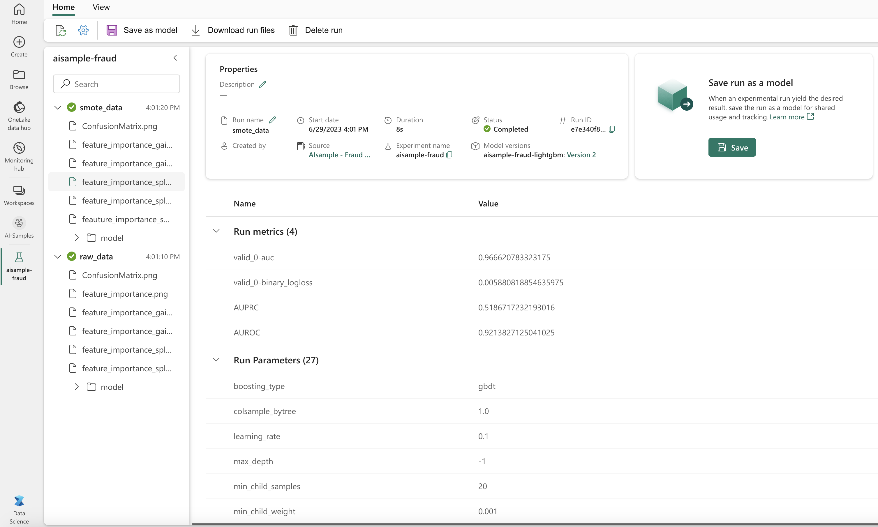
下圖顯示了在平衡資料集（ 版本2）上訓練模型的效能指標：

選擇 版本 1 以查看在不平衡資料集上訓練的模型的指標。當你比較這些指標時，你會發現用平衡資料集訓練的模型的 AUROC 較高。這些結果表示此模型較適合正確將 0 類別預測為 0，將類別 1 預測為 1。

步驟 5：註冊模型

使用 MLflow 註冊兩個模型：

# Register the model
registered_model_name = f"{EXPERIMENT_NAME}-lightgbm"

raw_model_uri = "runs:/{}/model".format(raw_run.info.run_id)
mlflow.register_model(raw_model_uri, registered_model_name)

smote_model_uri = "runs:/{}/model".format(smote_run.info.run_id)
mlflow.register_model(smote_model_uri, registered_model_name)

步驟 6：儲存預測結果

Microsoft Fabric使用者可以透過使用 PREDICT 可擴展函數來實作機器學習模型。此函數支援在任何計算引擎進行批次評分 (或批次推斷)。

你可以直接從 Microsoft Fabric 筆記本或模型的項目頁面產生批次預測。如需有關PREDICT的更多資訊，請參閱 Microsoft Fabric 中的PREDICT 模型評分。

載入效能較佳的模型 (版本 2) 以進行批次評分，並產生預測結果：

from synapse.ml.predict import MLFlowTransformer

spark.conf.set("spark.synapse.ml.predict.enabled", "true")

model = MLFlowTransformer(
    inputCols=feature_cols,
    outputCol="prediction",
    modelName=f"{EXPERIMENT_NAME}-lightgbm",
    modelVersion=2,
)

test_spark = spark.createDataFrame(data=test, schema=test.columns.to_list())

batch_predictions = model.transform(test_spark)

將預測儲存到 Lakehouse：

# Save the predictions to the lakehouse
batch_predictions.write.format("delta").mode("overwrite").save(f"{DATA_FOLDER}/predictions/batch_predictions")

意見反應

此頁面對您有幫助嗎？

Last updated on 2026-04-07