使用 PyTorch 定型數據分析模型

在本 教學課程的上一個階段中，我們已取得我們將用來使用 PyTorch 定型數據分析模型的數據集。 現在，是時候使用該數據了。

若要使用 PyTorch 定型數據分析模型，您需要完成下列步驟：

1. 載入數據。 如果您已完成本教學課程的上一個步驟，表示您已經處理過此作業。
2. 定義類神經網路。
3. 定義遺失函式。
4. 在訓練數據上訓練模型。
5. 在測試數據上測試網路。

定義類神經網路

在本教學課程中，您將建置具有三個線性圖層的基本類神經網路模型。 模型的結構如下所示：

Linear -> ReLU -> Linear -> ReLU -> Linear

線性層會將線性轉換套用至傳入數據。 您必須指定輸入特徵的數目，以及應該對應至類別數目的輸出特徵數目。

ReLU 層是一種啟用函數，用於將所有傳入特徵定義為 0 或大於 0。 因此，套用 ReLU 層時，小於 0 的任何數位會變更為零，而其他數位則維持不變。 我們會在兩個隱藏層上套用激活層，而在最後一個線性層上不會套用激活層。

模型參數

模型參數取決於我們的目標和定型數據。 輸入大小取決於我們饋送模型的功能數目， 在我們的案例中為 4 個。 輸出大小為三，因為有三種可能類型的虹膜。

有三個線性層， (4,24) -> (24,24) -> (24,3)網路會有744個權重（96+576+72）。

學習速率（lr）會設定控制您如何調整網路的權重以對應於損失梯度。 越低，訓練的速度越慢。 在本教學課程中，您會將 lr 設定為 0.01。

網路的運作方式為何？

在這裡，我們要建置轉送網路。 在訓練過程中，網路會通過所有層處理輸入、計算損失，以瞭解影像的預測標籤與正確標籤的差距，並將梯度回傳至網路，以更新層的權重。 透過逐一查看龐大的輸入數據集，網路將會「學習」設定其權數，以達到最佳結果。

正向函式會計算損失函式的值，即反向函式會計算可學習參數的梯度。 當您使用 PyTorch 建立神經網路時，只需要定義正向函式。 會自動定義回溯函式。

1. 將下列程式代碼 DataClassifier.py 複製到 Visual Studio 中的 檔案，以定義模型參數和神經網路。

# Define model parameters 
input_size = list(input.shape)[1]   # = 4. The input depends on how many features we initially feed the model. In our case, there are 4 features for every predict value  
learning_rate = 0.01 
output_size = len(labels)           # The output is prediction results for three types of Irises.  


# Define neural network 
class Network(nn.Module): 
   def __init__(self, input_size, output_size): 
       super(Network, self).__init__() 
        
       self.layer1 = nn.Linear(input_size, 24) 
       self.layer2 = nn.Linear(24, 24) 
       self.layer3 = nn.Linear(24, output_size) 


   def forward(self, x): 
       x1 = F.relu(self.layer1(x)) 
       x2 = F.relu(self.layer2(x1)) 
       x3 = self.layer3(x2) 
       return x3 
 
# Instantiate the model 
model = Network(input_size, output_size) 

您也必須根據電腦上的可用裝置來定義執行裝置。 PyTorch 沒有 GPU 專用連結庫，但您可以手動定義執行裝置。 如果你的計算機上有 Nvidia GPU，則裝置將是 Nvidia GPU；如果沒有，則將使用 CPU。

2. 複製下列程式代碼以定義執行裝置：

# Define your execution device 
device = torch.device("cuda:0" if torch.cuda.is_available() else "cpu") 
print("The model will be running on", device, "device\n") 
model.to(device)    # Convert model parameters and buffers to CPU or Cuda 

3. 在最後一個步驟中，定義用來儲存模型的函式：

# Function to save the model 
def saveModel(): 
    path = "./NetModel.pth" 
    torch.save(model.state_dict(), path) 

備註

有興趣深入瞭解使用 PyTorch 的類神經網路嗎？ 請參閱 PyTorch 檔。

定義遺失函式

損失函式會計算估計輸出距離目標距離的值。 主要目標是透過神經網路中的反向傳播調整加權向量值，以減少損失函式的值。

損失值與模型精確度不同。 損失函數表示我們的模型在訓練集上每次優化迭代後的表現。 模型的精確度會計算在測試數據上，並顯示正確預測的百分比。

在 PyTorch 中，類神經網路套件包含各種損失函式，形成深度神經網路的建置組塊。 如果您想要深入了解這些細節，請參考上述註記。 在這裡，我們將使用針對這類分類進行優化的現有函式，並使用分類交叉熵損失函式和 Adam 優化器。 在優化器中，學習率（lr）控制著您在根據損失梯度調整網路權重的程度。 您將在這裡將它設定為 0.001 - 值越低，訓練速度會比較慢。

1. 將下列程式代碼 DataClassifier.py 複製到 Visual Studio 中的 檔案，以定義遺失函式和優化器。

# Define the loss function with Classification Cross-Entropy loss and an optimizer with Adam optimizer
loss_fn = nn.CrossEntropyLoss()
optimizer = Adam(model.parameters(), lr=0.001, weight_decay=0.0001)

在訓練數據上訓練模型。

若要訓練模型，您必須遍歷我們的資料迭代器，將輸入饋送至神經網路並進行優化。 若要驗證結果，您只需在每次訓練迭代之後，將預測的標籤與驗證數據集中的實際標籤進行比較。

程序會顯示每個 epoch 的訓練損失、驗證損失和模型的準確率，或者在訓練集上的每次完整迭代中顯示。 它會以最高的準確率來儲存模型，經過10個訓練週期後，程式會顯示最終的準確率。

1. 將下列程式代碼新增至 DataClassifier.py 檔案

# Training Function 
def train(num_epochs): 
    best_accuracy = 0.0 
     
    print("Begin training...") 
    for epoch in range(1, num_epochs+1): 
        running_train_loss = 0.0 
        running_accuracy = 0.0 
        running_vall_loss = 0.0 
        total = 0 
 
        # Training Loop 
        for data in train_loader: 
        #for data in enumerate(train_loader, 0): 
            inputs, outputs = data  # get the input and real species as outputs; data is a list of [inputs, outputs] 
            optimizer.zero_grad()   # zero the parameter gradients          
            predicted_outputs = model(inputs)   # predict output from the model 
            train_loss = loss_fn(predicted_outputs, outputs)   # calculate loss for the predicted output  
            train_loss.backward()   # backpropagate the loss 
            optimizer.step()        # adjust parameters based on the calculated gradients 
            running_train_loss +=train_loss.item()  # track the loss value 
 
        # Calculate training loss value 
        train_loss_value = running_train_loss/len(train_loader) 
 
        # Validation Loop 
        with torch.no_grad(): 
            model.eval() 
            for data in validate_loader: 
               inputs, outputs = data 
               predicted_outputs = model(inputs) 
               val_loss = loss_fn(predicted_outputs, outputs) 
             
               # The label with the highest value will be our prediction 
               _, predicted = torch.max(predicted_outputs, 1) 
               running_vall_loss += val_loss.item()  
               total += outputs.size(0) 
               running_accuracy += (predicted == outputs).sum().item() 
 
        # Calculate validation loss value 
        val_loss_value = running_vall_loss/len(validate_loader) 
                
        # Calculate accuracy as the number of correct predictions in the validation batch divided by the total number of predictions done.  
        accuracy = (100 * running_accuracy / total)     
 
        # Save the model if the accuracy is the best 
        if accuracy > best_accuracy: 
            saveModel() 
            best_accuracy = accuracy 
         
        # Print the statistics of the epoch 
        print('Completed training batch', epoch, 'Training Loss is: %.4f' %train_loss_value, 'Validation Loss is: %.4f' %val_loss_value, 'Accuracy is %d %%' % (accuracy))

在測試數據上測試模型。

既然我們已定型模型，就可以使用測試數據集來測試模型。

我們將新增兩個測試函式。 第一個測試您在上一個部分中儲存的模型。 它會使用 45 個項目的測試數據集來測試模型，並顯示模型的精確度。 第二個是選擇性函式，用來測試模型預測三種虹膜物種中每一種的信心，其代表每個物種成功分類的機率。

1. 將下列程式碼新增至 DataClassifier.py 檔案。

# Function to test the model 
def test(): 
    # Load the model that we saved at the end of the training loop 
    model = Network(input_size, output_size) 
    path = "NetModel.pth" 
    model.load_state_dict(torch.load(path)) 
     
    running_accuracy = 0 
    total = 0 
 
    with torch.no_grad(): 
        for data in test_loader: 
            inputs, outputs = data 
            outputs = outputs.to(torch.float32) 
            predicted_outputs = model(inputs) 
            _, predicted = torch.max(predicted_outputs, 1) 
            total += outputs.size(0) 
            running_accuracy += (predicted == outputs).sum().item() 
 
        print('Accuracy of the model based on the test set of', test_split ,'inputs is: %d %%' % (100 * running_accuracy / total))    
 
 
# Optional: Function to test which species were easier to predict  
def test_species(): 
    # Load the model that we saved at the end of the training loop 
    model = Network(input_size, output_size) 
    path = "NetModel.pth" 
    model.load_state_dict(torch.load(path)) 
     
    labels_length = len(labels) # how many labels of Irises we have. = 3 in our database. 
    labels_correct = list(0. for i in range(labels_length)) # list to calculate correct labels [how many correct setosa, how many correct versicolor, how many correct virginica] 
    labels_total = list(0. for i in range(labels_length))   # list to keep the total # of labels per type [total setosa, total versicolor, total virginica] 
  
    with torch.no_grad(): 
        for data in test_loader: 
            inputs, outputs = data 
            predicted_outputs = model(inputs) 
            _, predicted = torch.max(predicted_outputs, 1) 
             
            label_correct_running = (predicted == outputs).squeeze() 
            label = outputs[0] 
            if label_correct_running.item():  
                labels_correct[label] += 1 
            labels_total[label] += 1  
  
    label_list = list(labels.keys()) 
    for i in range(output_size): 
        print('Accuracy to predict %5s : %2d %%' % (label_list[i], 100 * labels_correct[i] / labels_total[i])) 

最後，讓我們新增主要程序代碼。 這會起始模型定型、儲存模型，並在畫面上顯示結果。 我們只會在訓練集上執行兩次[num_epochs = 25]迭代，因此訓練過程不會花費太長的時間。

2. 將下列程式碼新增至 DataClassifier.py 檔案。

if __name__ == "__main__": 
    num_epochs = 10
    train(num_epochs) 
    print('Finished Training\n') 
    test() 
    test_species() 

讓我們執行測試！ 請確定頂端工具列中的下拉選單設定為 Debug。 如果您的裝置是64位，請將Solution Platform變更為x64，如果您的裝置是32位，請將Solution Platform變更為，以在您的本機電腦上執行專案。

3. 若要執行專案，請按下 Start Debugging 工具列上的按鈕，或按 F5。

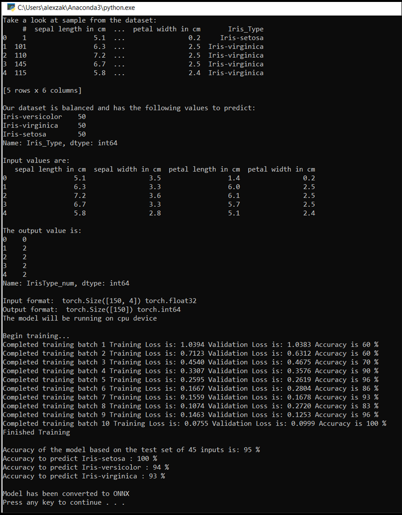
主控台視窗會彈出，您將會看到訓練過程。 如您所定義，將會列印每一個 Epoch 的遺失值。 預期遺失值會隨著每個迴圈而減少。

定型完成後，您應該會看到類似下面的輸出。 您的數值不會完全相同 - 訓練取決於許多因素，因此不會一律產生相同的結果，但看起來應該會類似。

後續步驟

既然我們有分類模型，下一個步驟是 將模型轉換成 ONNX 格式。