使用 PyTorch 將影像分類器模型定型

注意

為了獲得更大的功能， PyTorch 也可以與 Windows 上的 DirectML 搭配使用。

在本教學課程的上一個階段中，我們取得了我們將用來使用 PyTorch 定型影像分類器的數據集。 現在，是時候使用該數據了。

若要使用 PyTorch 定型影像分類器，您需要完成下列步驟：

1. 載入數據。 如果您已完成本教學課程的上一個步驟，表示您已經處理過此作業。
2. 定義卷積類神經網路。
3. 定義遺失函式。
4. 在訓練數據上訓練模型。
5. 在測試數據上測試網路。

定義卷積類神經網路。

若要使用 PyTorch 建置神經網路，您將使用 torch.nn 套件。 此套件包含模組、可延伸類別，以及建置神經網路所需的所有元件。

在這裡，您將建置基本的 捲積神經網路 （CNN），以分類來自CIFAR10數據集的影像。

CNN 是類神經網路，定義為多層神經網路，其設計目的是要偵測數據中的複雜特徵。 它們最常用於電腦視覺應用程式。

我們的網路將採用下列 14 層的結構：

Conv -> BatchNorm -> ReLU -> Conv -> BatchNorm -> ReLU -> MaxPool -> Conv -> BatchNorm -> ReLU -> Conv -> BatchNorm -> ReLU -> Linear。

捲積層

捲積層是CNN的主要層，可協助我們偵測影像中的特徵。 每個層都有數目的通道來偵測影像中的特定功能，以及定義所偵測功能大小的一些核心。 因此，具有 64 個通道和核心大小 3 x 3 的捲積層會偵測到 64 個不同的特徵，每個大小為 3 x 3。 當您定義捲積層時，您會提供通道內數目、輸出通道數目和核心大小。 層次中的輸出通道數目可作為下一層的輸入通道數目。

例如：具有輸入通道=3、輸出通道=10 且核心大小=6 的捲積層會將 RGB 影像（3 個通道）作為輸入，並將 10 個特徵檢測器套用至圖像，其中核心大小為 6x6。 較小的核心大小可減少計算時間和權數共用。

其他圖層

我們的網路涉及下列其他層：

• 此 ReLU 層是激活函數，可將所有輸入特徵定義為 0 或更大。 當您套用此圖層時，小於 0 的任何數位會變更為零，而其他數位則維持不變。
• 圖層 BatchNorm2d 會在輸入上套用正規化，以具有零平均數和單位變異數，並增加網路精確度。
• 圖層 MaxPool 將協助我們確保影像中物件的位置不會影響神經網路偵測其特定特徵的能力。
• 此 Linear 層是我們網路中的最終層，它會計算每個類別的分數。 在CIFAR10數據集中，有十個標籤類別。 具有最高分數的標籤將會是模型預測的標籤。 在線性圖層中，您必須指定輸入特徵的數目，以及應該對應至類別數目的輸出特徵數目。

類神經網路如何運作？

CNN 是一個轉送網路。 在訓練過程中，網路會通過所有層處理輸入、計算損失，以瞭解影像的預測標籤與正確標籤的差距，並將梯度回傳至網路，以更新層的權重。 透過逐一查看龐大的輸入數據集，網路將會「學習」設定其權數，以達到最佳結果。

正向函式會計算遺失函式的值，而向後函式會計算可學習參數的漸層。 當您使用 PyTorch 建立神經網路時，只需要定義正向函式。 會自動定義回溯函式。

1. 將下列程式代碼複製到 PyTorchTraining.py Visual Studio 中的檔案，以定義 CCN。

import torch
import torch.nn as nn
import torchvision
import torch.nn.functional as F

# Define a convolution neural network
class Network(nn.Module):
    def __init__(self):
        super(Network, self).__init__()
        
        self.conv1 = nn.Conv2d(in_channels=3, out_channels=12, kernel_size=5, stride=1, padding=1)
        self.bn1 = nn.BatchNorm2d(12)
        self.conv2 = nn.Conv2d(in_channels=12, out_channels=12, kernel_size=5, stride=1, padding=1)
        self.bn2 = nn.BatchNorm2d(12)
        self.pool = nn.MaxPool2d(2,2)
        self.conv4 = nn.Conv2d(in_channels=12, out_channels=24, kernel_size=5, stride=1, padding=1)
        self.bn4 = nn.BatchNorm2d(24)
        self.conv5 = nn.Conv2d(in_channels=24, out_channels=24, kernel_size=5, stride=1, padding=1)
        self.bn5 = nn.BatchNorm2d(24)
        self.fc1 = nn.Linear(24*10*10, 10)

    def forward(self, input):
        output = F.relu(self.bn1(self.conv1(input)))      
        output = F.relu(self.bn2(self.conv2(output)))     
        output = self.pool(output)                        
        output = F.relu(self.bn4(self.conv4(output)))     
        output = F.relu(self.bn5(self.conv5(output)))     
        output = output.view(-1, 24*10*10)
        output = self.fc1(output)

        return output

# Instantiate a neural network model 
model = Network()

注意

有興趣深入瞭解使用 PyTorch 的類神經網路嗎？ 查看 PyTorch 文件

定義遺失函式

損失函式會計算估計輸出距離目標距離的值。 主要目標是透過神經網路中的反向傳播調整加權向量值，以減少損失函式的值。

損失值與模型精確度不同。 損失函數讓我們了解模型在訓練集上每次優化迭代後的性能表現。 模型的精確度會計算在測試數據上，並顯示正確預測的百分比。

在 PyTorch 中，類神經網路套件包含各種損失函式，形成深度神經網路的建置組塊。 在本教學課程中，您將使用基於分類交叉熵損失和 Adam 優化器的損失函式來定義分類損失函式。 學習速率（lr）設定您調整網路權重時對損失梯度影響程度的控制。 您將將其設定為 0.001。 越低，訓練的速度越慢。

1. 將下列程式代碼 PyTorchTraining.py 複製到 Visual Studio 中的 檔案，以定義遺失函式和優化器。

from torch.optim import Adam
 
# Define the loss function with Classification Cross-Entropy loss and an optimizer with Adam optimizer
loss_fn = nn.CrossEntropyLoss()
optimizer = Adam(model.parameters(), lr=0.001, weight_decay=0.0001)

在訓練數據上訓練模型。

若要訓練模型，您必須遍歷我們的資料迭代器，將輸入饋送至神經網路並進行優化。 PyTorch 沒有專用的 GPU 使用連結庫，但您可以手動定義執行裝置。 如果計算機上存在，則裝置會是 Nvidia GPU，如果不存在，則為 CPU。

1. 將下列程式代碼新增至 PyTorchTraining.py 檔案

from torch.autograd import Variable

# Function to save the model
def saveModel():
    path = "./myFirstModel.pth"
    torch.save(model.state_dict(), path)

# Function to test the model with the test dataset and print the accuracy for the test images
def testAccuracy():
    
    model.eval()
    accuracy = 0.0
    total = 0.0
    device = torch.device("cuda:0" if torch.cuda.is_available() else "cpu")
    
    with torch.no_grad():
        for data in test_loader:
            images, labels = data
            # run the model on the test set to predict labels
            outputs = model(images.to(device))
            # the label with the highest energy will be our prediction
            _, predicted = torch.max(outputs.data, 1)
            total += labels.size(0)
            accuracy += (predicted == labels.to(device)).sum().item()
    
    # compute the accuracy over all test images
    accuracy = (100 * accuracy / total)
    return(accuracy)


# Training function. We simply have to loop over our data iterator and feed the inputs to the network and optimize.
def train(num_epochs):
    
    best_accuracy = 0.0

    # Define your execution device
    device = torch.device("cuda:0" if torch.cuda.is_available() else "cpu")
    print("The model will be running on", device, "device")
    # Convert model parameters and buffers to CPU or Cuda
    model.to(device)

    for epoch in range(num_epochs):  # loop over the dataset multiple times
        running_loss = 0.0
        running_acc = 0.0

        for i, (images, labels) in enumerate(train_loader, 0):
            
            # get the inputs
            images = Variable(images.to(device))
            labels = Variable(labels.to(device))

            # zero the parameter gradients
            optimizer.zero_grad()
            # predict classes using images from the training set
            outputs = model(images)
            # compute the loss based on model output and real labels
            loss = loss_fn(outputs, labels)
            # backpropagate the loss
            loss.backward()
            # adjust parameters based on the calculated gradients
            optimizer.step()

            # Let's print statistics for every 1,000 images
            running_loss += loss.item()     # extract the loss value
            if i % 1000 == 999:    
                # print every 1000 (twice per epoch) 
                print('[%d, %5d] loss: %.3f' %
                      (epoch + 1, i + 1, running_loss / 1000))
                # zero the loss
                running_loss = 0.0

        # Compute and print the average accuracy fo this epoch when tested over all 10000 test images
        accuracy = testAccuracy()
        print('For epoch', epoch+1,'the test accuracy over the whole test set is %d %%' % (accuracy))
        
        # we want to save the model if the accuracy is the best
        if accuracy > best_accuracy:
            saveModel()
            best_accuracy = accuracy

在測試數據上測試模型。

現在，您可以使用來自測試集的影像批次來測試模型。

1. 將下列程式碼新增至 PyTorchTraining.py 檔案。

import matplotlib.pyplot as plt
import numpy as np

# Function to show the images
def imageshow(img):
    img = img / 2 + 0.5     # unnormalize
    npimg = img.numpy()
    plt.imshow(np.transpose(npimg, (1, 2, 0)))
    plt.show()


# Function to test the model with a batch of images and show the labels predictions
def testBatch():
    # get batch of images from the test DataLoader  
    images, labels = next(iter(test_loader))

    # show all images as one image grid
    imageshow(torchvision.utils.make_grid(images))
   
    # Show the real labels on the screen 
    print('Real labels: ', ' '.join('%5s' % classes[labels[j]] 
                               for j in range(batch_size)))
  
    # Let's see what if the model identifiers the  labels of those example
    outputs = model(images)
    
    # We got the probability for every 10 labels. The highest (max) probability should be correct label
    _, predicted = torch.max(outputs, 1)
    
    # Let's show the predicted labels on the screen to compare with the real ones
    print('Predicted: ', ' '.join('%5s' % classes[predicted[j]] 
                              for j in range(batch_size)))

最後，讓我們新增主要程序代碼。 這會起始模型定型、儲存模型，並在畫面上顯示結果。 我們只會在訓練集上執行兩次[train(2)]迭代，因此訓練過程不會花費太長的時間。

2. 將下列程式碼新增至 PyTorchTraining.py 檔案。

if __name__ == "__main__":
    
    # Let's build our model
    train(5)
    print('Finished Training')

    # Test which classes performed well
    testAccuracy()
    
    # Let's load the model we just created and test the accuracy per label
    model = Network()
    path = "myFirstModel.pth"
    model.load_state_dict(torch.load(path))

    # Test with batch of images
    testBatch()

讓我們執行測試！ 請確定頂端工具列中的下拉功能表設定為 [偵錯]。 如果您的裝置是 64 位元，請將方案平臺變更為 x64，以便在本機電腦上執行專案；如果您的裝置是 32 位元，請將方案平臺變更為 x86。

選擇 epoch 數（完整通過訓練數據集的次數）等於兩個（[train(2)]）會導致對包含 10,000 張影像的整個測試數據集進行兩次的遍歷。 完成在第 8 代 Intel CPU 上的訓練大約需要 20 分鐘，模型在十個標籤的分類中應能達到約 65% 的成功率。

3. 若要執行專案，按一下工具列上的 [開始偵錯] 按鈕，或按下 F5。

控制台視窗將會彈出，並且能夠看到訓練的過程。

如您所定義，損失值會每 1,000 批影像輸出一次，或在每次訓練集的迭代中執行五次。 您預期遺失值會隨著每個循環而減少。

您也會在每次迭代之後看到模型的正確性。 模型精確度與損失值不同。 損失函數讓我們了解模型在訓練集上每次優化迭代後的性能表現。 模型的精確度會計算在測試數據上，並顯示正確預測的百分比。 在我們的情況中，它將告訴我們在每次訓練迭代後，10,000 個影像測試集中有多少個影像能夠被正確分類。

定型完成後，您應該會看到類似下面的輸出。 您的數位不會完全相同 - 根據許多因素進行編碼，而且不會一律傳回識別結果，但看起來應該類似。

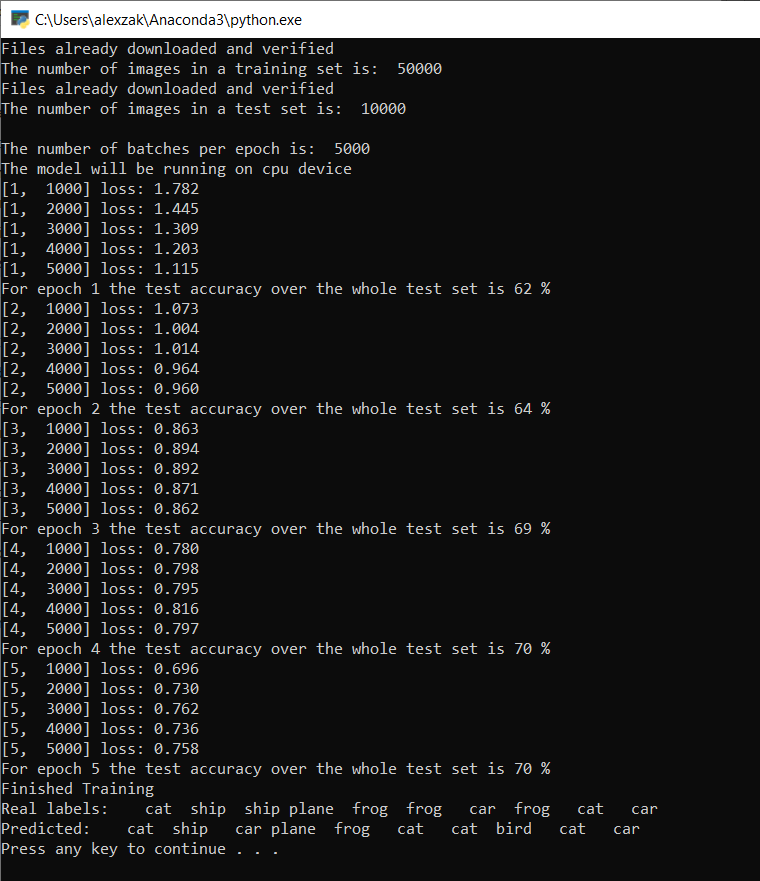
執行 5 個 Epoch 之後，模型成功率為 70%。 這是在短時間內定型的基本模型的良好結果！

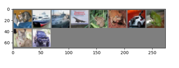
使用包含10張影像的批次進行測試，模型正確識別了其中7張影像。 完全不壞，而且與模型成功率一致。

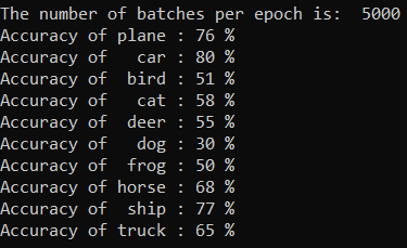
您可以檢查我們的模型最擅長預測哪些類別。 簡單地將下列程式代碼添加並運行：

4. 選擇性 - 將下列 testClassess 函式新增至 PyTorchTraining.py 檔案，在 main 函式內新增此函 testClassess() 式的呼叫 - __name__ == "__main__"。

# Function to test what classes performed well
def testClassess():
    class_correct = list(0. for i in range(number_of_labels))
    class_total = list(0. for i in range(number_of_labels))
    with torch.no_grad():
        for data in test_loader:
            images, labels = data
            outputs = model(images)
            _, predicted = torch.max(outputs, 1)
            c = (predicted == labels).squeeze()
            for i in range(batch_size):
                label = labels[i]
                class_correct[label] += c[i].item()
                class_total[label] += 1

    for i in range(number_of_labels):
        print('Accuracy of %5s : %2d %%' % (
            classes[i], 100 * class_correct[i] / class_total[i]))

輸出如下所示：

後續步驟

既然我們有分類模型，下一個步驟是將 模型轉換成 ONNX 格式