Note
Access to this page requires authorization. You can try signing in or changing directories.
Access to this page requires authorization. You can try changing directories.
This tutorial presents an end-to-end example of a Synapse Data Science workflow in Microsoft Fabric. The scenario builds a model for online book recommendations.
This tutorial covers these steps:
- Upload the data into a lakehouse
- Perform exploratory analysis on the data
- Train a model, and log it with MLflow
- Load the model and make predictions
Many types of recommendation algorithms are available. This tutorial uses the Alternating Least Squares (ALS) matrix factorization algorithm. ALS is a model-based collaborative filtering algorithm.

ALS tries to estimate the ratings matrix R as the product of two lower-rank matrices, U and V. Here, R = U * Vt. Typically, these approximations are called factor matrices.
The ALS algorithm is iterative. Each iteration holds one of the factor matrices constant, while it solves the other using the method of least squares. It then holds that newly solved factor matrix constant while it solves the other factor matrix.

Prerequisites
Get a Microsoft Fabric subscription. Or, sign up for a free Microsoft Fabric trial.
Sign in to Microsoft Fabric.
Switch to Fabric by using the experience switcher on the lower-left side of your home page.

- If necessary, create a Microsoft Fabric lakehouse as described in Create a lakehouse in Microsoft Fabric.
Follow along in a notebook
Choose one of these options to follow along in a notebook:
- Open and run the built-in notebook.
- Upload your notebook from GitHub.
Open the built-in notebook
The sample Book recommendation notebook accompanies this tutorial.
To open the sample notebook for this tutorial, follow the instructions in Prepare your system for data science tutorials.
Make sure to attach a lakehouse to the notebook before you start running code.
Import the notebook from GitHub
The AIsample - Book Recommendation.ipynb notebook accompanies this tutorial.
To open the accompanying notebook for this tutorial, follow the instructions in Prepare your system for data science tutorials to import the notebook to your workspace.
If you'd rather copy and paste the code from this page, you can create a new notebook.
Be sure to attach a lakehouse to the notebook before you start running code.
Step 1: Load the data
The book recommendation dataset in this scenario consists of three separate datasets:
Books.csv: An International Standard Book Number (ISBN) identifies each book, with invalid dates already removed. The dataset also includes the title, author, and publisher. For a book with multiple authors, the Books.csv file lists only the first author. URLs point to Amazon website resources for the cover images, in three sizes.
ISBN Book-Title Book-Author Year-Of-Publication Publisher Image-URL-S Image-URL-M Image-URL-l 0195153448 Classical Mythology Mark P. O. Morford 2002 Oxford University Press http://images.amazon.com/images/P/0195153448.01.THUMBZZZ.jpg http://images.amazon.com/images/P/0195153448.01.MZZZZZZZ.jpg http://images.amazon.com/images/P/0195153448.01.LZZZZZZZ.jpg 0002005018 Clara Callan Richard Bruce Wright 2001 HarperFlamingo Canada http://images.amazon.com/images/P/0002005018.01.THUMBZZZ.jpg http://images.amazon.com/images/P/0002005018.01.MZZZZZZZ.jpg http://images.amazon.com/images/P/0002005018.01.LZZZZZZZ.jpg Ratings.csv: Ratings for each book are either explicit (provided by users, on a scale of 1 to 10) or implicit (observed without user input, and indicated by 0).
User-ID ISBN Book-Rating 276725 034545104X 0 276726 0155061224 5 Users.csv: User IDs are anonymized and mapped to integers. Demographic data - for example, location and age - are provided, if available. If this data is unavailable, these values are
null.User-ID Location Age 1 "nyc new york usa" 2 "stockton california usa" 18.0
Define these parameters, so that you can use this notebook with different datasets:
IS_CUSTOM_DATA = False  # If True, the dataset has to be uploaded manually

USER_ID_COL = "User-ID"  # Must not be '_user_id' for this notebook to run successfully
ITEM_ID_COL = "ISBN"  # Must not be '_item_id' for this notebook to run successfully
ITEM_INFO_COL = (
    "Book-Title"  # Must not be '_item_info' for this notebook to run successfully
)
RATING_COL = (
    "Book-Rating"  # Must not be '_rating' for this notebook to run successfully
)
IS_SAMPLE = True  # If True, use only <SAMPLE_ROWS> rows of data for training; otherwise, use all data
SAMPLE_ROWS = 5000  # If IS_SAMPLE is True, use only this number of rows for training

DATA_FOLDER = "Files/book-recommendation/"  # Folder that contains the datasets
ITEMS_FILE = "Books.csv"  # File that contains the item information
USERS_FILE = "Users.csv"  # File that contains the user information
RATINGS_FILE = "Ratings.csv"  # File that contains the rating information

EXPERIMENT_NAME = "aisample-recommendation"  # MLflow experiment name
Download and store the data in a lakehouse
This code downloads the dataset, and then stores it in the lakehouse.
Important
Be sure to add a lakehouse to the notebook before you run it. Otherwise, you get an error.
if not IS_CUSTOM_DATA:
    # Download data files into a lakehouse if they don't exist
    import os, requests

    remote_url = "https://synapseaisolutionsa.z13.web.core.windows.net/data/Book-Recommendation-Dataset"
    file_list = ["Books.csv", "Ratings.csv", "Users.csv"]
    download_path = f"/lakehouse/default/{DATA_FOLDER}/raw"

    if not os.path.exists("/lakehouse/default"):
        raise FileNotFoundError(
            "Default lakehouse not found, please add a lakehouse and restart the session."
        )
    os.makedirs(download_path, exist_ok=True)
    for fname in file_list:
        if not os.path.exists(f"{download_path}/{fname}"):
            r = requests.get(f"{remote_url}/{fname}", timeout=30)
            with open(f"{download_path}/{fname}", "wb") as f:
                f.write(r.content)
    print("Downloaded demo data files into lakehouse.")
Set up the MLflow experiment tracking
Use this code to set up the MLflow experiment tracking. This example disables autologging. For more information, see the Autologging in Microsoft Fabric article.
# Set up MLflow for experiment tracking
import mlflow

mlflow.set_experiment(EXPERIMENT_NAME)
mlflow.autolog(disable=True)  # Disable MLflow autologging
Read data from the lakehouse
After you place the correct data in the lakehouse, read the three datasets into separate Spark DataFrames in the notebook. The file paths in this code use the parameters defined earlier.
df_items = (
    spark.read.option("header", True)
    .option("inferSchema", True)
    .csv(f"{DATA_FOLDER}/raw/{ITEMS_FILE}")
    .cache()
)

df_ratings = (
    spark.read.option("header", True)
    .option("inferSchema", True)
    .csv(f"{DATA_FOLDER}/raw/{RATINGS_FILE}")
    .cache()
)

df_users = (
    spark.read.option("header", True)
    .option("inferSchema", True)
    .csv(f"{DATA_FOLDER}/raw/{USERS_FILE}")
    .cache()
)
Step 2: Perform exploratory data analysis
Display raw data
Explore the DataFrames by using the display command. By using this command, you can view high-level DataFrame statistics and understand how different dataset columns relate to each other. Before you explore the datasets, use this code to import the required libraries:
import pyspark.sql.functions as F
from pyspark.ml.feature import StringIndexer
import matplotlib.pyplot as plt
import seaborn as sns
color = sns.color_palette()  # Adjusting plotting style
import pandas as pd  # DataFrames
Use this code to look at the DataFrame that contains the book data:
display(df_items, summary=True)
Add an _item_id column for later use. The _item_id value must be an integer for recommendation models. This code uses StringIndexer to transform ITEM_ID_COL to indices:
df_items = (
    StringIndexer(inputCol=ITEM_ID_COL, outputCol="_item_id")
    .setHandleInvalid("skip")
    .fit(df_items)
    .transform(df_items)
    .withColumn("_item_id", F.col("_item_id").cast("int"))
)
Display the DataFrame, and check whether the _item_id value increases monotonically and successively, as expected:
display(df_items.sort(F.col("_item_id").desc()))
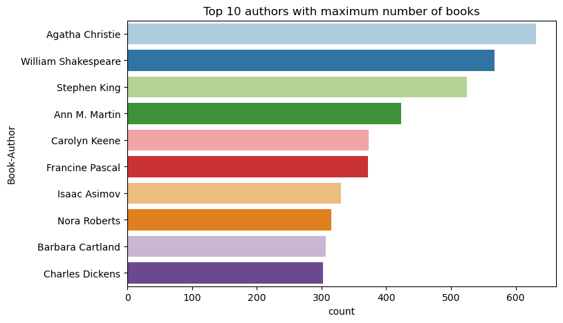
Use this code to plot the top 10 authors, by number of books written, in descending order. Agatha Christie is the leading author with more than 600 books, followed by William Shakespeare.
df_books = df_items.toPandas() # Create a pandas DataFrame from the Spark DataFrame for visualization
plt.figure(figsize=(8,5))
sns.countplot(y="Book-Author",palette = 'Paired', data=df_books,order=df_books['Book-Author'].value_counts().index[0:10])
plt.title("Top 10 authors with maximum number of books")
Next, display the DataFrame that contains the user data:
display(df_users, summary=True)
If a row has a missing User-ID value, drop that row. Missing values in a customized dataset don't cause problems.
df_users = df_users.dropna(subset=(USER_ID_COL))
display(df_users, summary=True)
Add a _user_id column for later use. For recommendation models, the _user_id value must be an integer. The following code sample uses StringIndexer to transform USER_ID_COL to indices.
The book dataset already has an integer User-ID column. However, adding a _user_id column for compatibility with different datasets makes this example more robust. Use this code to add the _user_id column:
df_users = (
    StringIndexer(inputCol=USER_ID_COL, outputCol="_user_id")
    .setHandleInvalid("skip")
    .fit(df_users)
    .transform(df_users)
    .withColumn("_user_id", F.col("_user_id").cast("int"))
)
display(df_users.sort(F.col("_user_id").desc()))
Use this code to view the rating data:
display(df_ratings, summary=True)
Obtain the distinct ratings, and save them for later use in a list named ratings:
ratings = [i[0] for i in df_ratings.select(RATING_COL).distinct().collect()]
print(ratings)
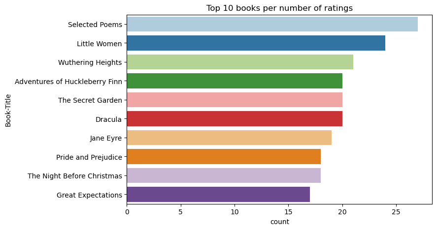
Use this code to show the top 10 books with the highest ratings:
plt.figure(figsize=(8,5))
sns.countplot(y="Book-Title",palette = 'Paired',data= df_books, order=df_books['Book-Title'].value_counts().index[0:10])
plt.title("Top 10 books per number of ratings")
According to the ratings, Selected Poems is the most popular book. Adventures of Huckleberry Finn, The Secret Garden, and Dracula have the same rating.
Merge data
Merge the three DataFrames into one DataFrame for a more comprehensive analysis:
df_all = df_ratings.join(df_users, USER_ID_COL, "inner").join(
    df_items, ITEM_ID_COL, "inner"
)
df_all_columns = [
    c for c in df_all.columns if c not in ["_user_id", "_item_id", RATING_COL]
]

# Reorder the columns to ensure that _user_id, _item_id, and Book-Rating are the first three columns
df_all = (
    df_all.select(["_user_id", "_item_id", RATING_COL] + df_all_columns)
    .withColumn("id", F.monotonically_increasing_id())
    .cache()
)

display(df_all)
Use this code to display a count of the distinct users, books, and interactions:
print(f"Total Users: {df_users.select('_user_id').distinct().count()}")
print(f"Total Items: {df_items.select('_item_id').distinct().count()}")
print(f"Total User-Item Interactions: {df_all.count()}")
Compute and plot the most popular items
Use this code to compute and display the top 10 most popular books:
# Compute top popular products
df_top_items = (
    df_all.groupby(["_item_id"])
    .count()
    .join(df_items, "_item_id", "inner")
    .sort(["count"], ascending=[0])
)

# Find top <topn> popular items
topn = 10
pd_top_items = df_top_items.limit(topn).toPandas()
pd_top_items.head(10)
Tip
Use the <topn> value for Popular or Top purchased recommendation sections.
# Plot top <topn> items
f, ax = plt.subplots(figsize=(10, 5))
plt.xticks(rotation="vertical")
sns.barplot(y=ITEM_INFO_COL, x="count", data=pd_top_items)
ax.tick_params(axis='x', rotation=45)
plt.xlabel("Number of Ratings for the Item")
plt.show()

Prepare training and test datasets
The ALS matrix requires some data preparation before training. Use this code sample to prepare the data. The code performs these actions:
- Cast the rating column to the correct type.
- Sample the training data with user ratings.
- Split the data into training and test datasets.
if IS_SAMPLE:
    # Must sort by '_user_id' before performing limit to ensure that ALS works normally
    # If training and test datasets have no common _user_id, ALS will fail
    df_all = df_all.sort("_user_id").limit(SAMPLE_ROWS)

# Cast the column into the correct type
df_all = df_all.withColumn(RATING_COL, F.col(RATING_COL).cast("float"))

# Using a fraction between 0 and 1 returns the approximate size of the dataset; for example, 0.8 means 80% of the dataset
# Rating = 0 means the user didn't rate the item, so it can't be used for training
# We use the 80% of the dataset with rating > 0 as the training dataset
fractions_train = {0: 0}
fractions_test = {0: 0}
for i in ratings:
    if i == 0:
        continue
    fractions_train[i] = 0.8
    fractions_test[i] = 1
# Training dataset
train = df_all.sampleBy(RATING_COL, fractions=fractions_train)

# Join with leftanti will select all rows from df_all with rating > 0 and not in the training dataset; for example, the remaining 20% of the dataset
# test dataset
test = df_all.join(train, on="id", how="leftanti").sampleBy(
    RATING_COL, fractions=fractions_test
)
Sparsity refers to sparse feedback data, which can't identify similarities in users' interests. For a better understanding of both the data and the current problem, use this code to compute the dataset sparsity:
# Compute the sparsity of the dataset
def get_mat_sparsity(ratings):
    # Count the total number of ratings in the dataset - used as numerator
    count_nonzero = ratings.select(RATING_COL).count()
    print(f"Number of rows: {count_nonzero}")

    # Count the total number of distinct user_id and distinct product_id - used as denominator
    total_elements = (
        ratings.select("_user_id").distinct().count()
        * ratings.select("_item_id").distinct().count()
    )

    # Calculate the sparsity by dividing the numerator by the denominator
    sparsity = (1.0 - (count_nonzero * 1.0) / total_elements) * 100
    print("The ratings DataFrame is ", "%.4f" % sparsity + "% sparse.")

get_mat_sparsity(df_all)
# Check the ID range
# ALS supports only values in the integer range
print(f"max user_id: {df_all.agg({'_user_id': 'max'}).collect()[0][0]}")
print(f"max user_id: {df_all.agg({'_item_id': 'max'}).collect()[0][0]}")
Step 3: Develop and train the model
Train an ALS model to give users personalized recommendations.
Define the model
Spark ML provides a convenient API for building the ALS model. However, the model doesn't reliably handle problems like data sparsity and cold start (making recommendations when the users or items are new). To improve model performance, combine cross-validation and automatic hyperparameter tuning.
Use this code to import the libraries required for model training and evaluation:
# Import Spark required libraries
from pyspark.ml.evaluation import RegressionEvaluator
from pyspark.ml.recommendation import ALS
from pyspark.ml.tuning import ParamGridBuilder, CrossValidator, TrainValidationSplit

# Specify the training parameters
num_epochs = 1  # Number of epochs; here we use 1 to reduce the training time
rank_size_list = [64]  # The values of rank in ALS for tuning
reg_param_list = [0.01, 0.1]  # The values of regParam in ALS for tuning
model_tuning_method = "TrainValidationSplit"  # TrainValidationSplit or CrossValidator
# Build the recommendation model by using ALS on the training data
# We set the cold start strategy to 'drop' to ensure that we don't get NaN evaluation metrics
als = ALS(
    maxIter=num_epochs,
    userCol="_user_id",
    itemCol="_item_id",
    ratingCol=RATING_COL,
    coldStartStrategy="drop",
    implicitPrefs=False,
    nonnegative=True,
)
Tune model hyperparameters
The next code sample constructs a parameter grid to help search over the hyperparameters. The code also creates a regression evaluator that uses the root-mean-square error (RMSE) as the evaluation metric:
#  Construct a grid search to select the best values for the training parameters
param_grid = (
    ParamGridBuilder()
    .addGrid(als.rank, rank_size_list)
    .addGrid(als.regParam, reg_param_list)
    .build()
)

print("Number of models to be tested: ", len(param_grid))

# Define the evaluator and set the loss function to the RMSE
evaluator = RegressionEvaluator(
    metricName="rmse", labelCol=RATING_COL, predictionCol="prediction"
)
The next code sample initiates different model tuning methods based on the preconfigured parameters. For more information about model tuning, see ML Tuning: model selection and hyperparameter tuning at the Apache Spark website.
# Build cross-validation by using CrossValidator and TrainValidationSplit
if model_tuning_method == "CrossValidator":
    tuner = CrossValidator(
        estimator=als,
        estimatorParamMaps=param_grid,
        evaluator=evaluator,
        numFolds=5,
        collectSubModels=True,
    )
elif model_tuning_method == "TrainValidationSplit":
    tuner = TrainValidationSplit(
        estimator=als,
        estimatorParamMaps=param_grid,
        evaluator=evaluator,
        # 80% of the training data will be used for training; 20% for validation
        trainRatio=0.8,
        collectSubModels=True,
    )
else:
    raise ValueError(f"Unknown model_tuning_method: {model_tuning_method}")
Evaluate the model
Evaluate models against the test data. A well-trained model has high metrics on the dataset.
An overfitted model might need more training data or a reduction of some redundant features. You might need to change the model architecture or fine tune its parameters.
Note
A negative R-squared metric value indicates that the trained model performs worse than a horizontal straight line. This finding suggests that the trained model doesn't explain the data.
Use this code to define an evaluation function:
def evaluate(model, data, verbose=0):
    """
    Evaluate the model by computing rmse, mae, r2, and variance over the data.
    """

    predictions = model.transform(data).withColumn(
        "prediction", F.col("prediction").cast("double")
    )

    if verbose > 1:
        # Show 10 predictions
        predictions.select("_user_id", "_item_id", RATING_COL, "prediction").limit(
            10
        ).show()

    # Initialize the regression evaluator
    evaluator = RegressionEvaluator(predictionCol="prediction", labelCol=RATING_COL)

    _evaluator = lambda metric: evaluator.setMetricName(metric).evaluate(predictions)
    rmse = _evaluator("rmse")
    mae = _evaluator("mae")
    r2 = _evaluator("r2")
    var = _evaluator("var")

    if verbose > 0:
        print(f"RMSE score = {rmse}")
        print(f"MAE score = {mae}")
        print(f"R2 score = {r2}")
        print(f"Explained variance = {var}")

    return predictions, (rmse, mae, r2, var)
Track the experiment by using MLflow
Use MLflow to track all the experiments and to log parameters, metrics, and models. To start model training and evaluation, use this code:
from mlflow.models.signature import infer_signature

with mlflow.start_run(run_name="als"):
    # Train models
    models = tuner.fit(train)
    best_metrics = {"RMSE": 10e6, "MAE": 10e6, "R2": 0, "Explained variance": 0}
    best_index = 0
    # Evaluate models
    # Log models, metrics, and parameters
    for idx, model in enumerate(models.subModels):
        with mlflow.start_run(nested=True, run_name=f"als_{idx}") as run:
            print("\nEvaluating on test data:")
            print(f"subModel No. {idx + 1}")
            predictions, (rmse, mae, r2, var) = evaluate(model, test, verbose=1)

            signature = infer_signature(
                train.select(["_user_id", "_item_id"]),
                predictions.select(["_user_id", "_item_id", "prediction"]),
            )
            print("log model:")
            mlflow.spark.log_model(
                model,
                f"{EXPERIMENT_NAME}-alsmodel",
                signature=signature,
                registered_model_name=f"{EXPERIMENT_NAME}-alsmodel",
                dfs_tmpdir="Files/spark",
            )
            print("log metrics:")
            current_metric = {
                "RMSE": rmse,
                "MAE": mae,
                "R2": r2,
                "Explained variance": var,
            }
            mlflow.log_metrics(current_metric)
            if rmse < best_metrics["RMSE"]:
                best_metrics = current_metric
                best_index = idx

            print("log parameters:")
            mlflow.log_params(
                {
                    "subModel_idx": idx,
                    "num_epochs": num_epochs,
                    "rank_size_list": rank_size_list,
                    "reg_param_list": reg_param_list,
                    "model_tuning_method": model_tuning_method,
                    "DATA_FOLDER": DATA_FOLDER,
                }
            )
    # Log the best model and related metrics and parameters to the parent run
    mlflow.spark.log_model(
        models.subModels[best_index],
        f"{EXPERIMENT_NAME}-alsmodel",
        signature=signature,
        registered_model_name=f"{EXPERIMENT_NAME}-alsmodel",
        dfs_tmpdir="Files/spark",
    )
    mlflow.log_metrics(best_metrics)
    mlflow.log_params(
        {
            "subModel_idx": idx,
            "num_epochs": num_epochs,
            "rank_size_list": rank_size_list,
            "reg_param_list": reg_param_list,
            "model_tuning_method": model_tuning_method,
            "DATA_FOLDER": DATA_FOLDER,
        }
    )
Select the experiment named aisample-recommendation from your workspace to view the logged information for the training run. If you change the experiment name, select the experiment that has the new name. The logged information resembles this image:

Step 4: Load the final model for scoring and make predictions
After you finish training the model and select the best model, load the model for scoring (sometimes called inferencing). This code loads the model and uses predictions to recommend the top 10 books for each user:
# Load the best model
# MLflow uses PipelineModel to wrap the original model, so we extract the original ALSModel from the stages
model_uri = f"models:/{EXPERIMENT_NAME}-alsmodel/1"
loaded_model = mlflow.spark.load_model(model_uri, dfs_tmpdir="Files/spark").stages[-1]

# Generate top 10 book recommendations for each user
userRecs = loaded_model.recommendForAllUsers(10)

# Represent the recommendations in an interpretable format
userRecs = (
    userRecs.withColumn("rec_exp", F.explode("recommendations"))
    .select("_user_id", F.col("rec_exp._item_id"), F.col("rec_exp.rating"))
    .join(df_items.select(["_item_id", "Book-Title"]), on="_item_id")
)
userRecs.limit(10).show()
The output resembles this table:
| _item_id | _user_id | rating | Book-Title |
|---|---|---|---|
| 44865 | 7 | 7.9996786 | Lasher: Lives of ... |
| 786 | 7 | 6.2255826 | The Piano Man's D... |
| 45330 | 7 | 4.980466 | State of Mind |
| 38960 | 7 | 4.980466 | All He Ever Wanted |
| 125415 | 7 | 4.505084 | Harry Potter and ... |
| 44939 | 7 | 4.3579073 | Taltos: Lives of ... |
| 175247 | 7 | 4.3579073 | The Bonesetter's ... |
| 170183 | 7 | 4.228735 | Living the Simple... |
| 88503 | 7 | 4.221206 | Island of the Blu... |
| 32894 | 7 | 3.9031885 | Winter Solstice |
Save the predictions to the lakehouse
Use this code to write the recommendations back to the lakehouse:
# Code to save userRecs into the lakehouse
userRecs.write.format("delta").mode("overwrite").save(
    f"{DATA_FOLDER}/predictions/userRecs"
)