Note
Access to this page requires authorization. You can try signing in or changing directories.
Access to this page requires authorization. You can try changing directories.
This tutorial presents an end-to-end example of a Synapse Data Science workflow in Microsoft Fabric. The scenario builds a forecasting model that uses historical sales data to predict product category sales at a superstore.
Forecasting is a crucial asset in sales. It combines historical data and predictive methods to provide insights about future trends. Forecasting can analyze past sales to identify patterns. It can also learn from consumer behavior to optimize inventory, production, and marketing strategies. This proactive approach enhances adaptability, responsiveness, and overall business performance in a dynamic marketplace.
This tutorial covers these steps:
- Load the data
- Use exploratory data analysis to understand and process the data
- Train a machine learning model with an open-source software package
- Track experiments with MLflow and the Fabric autologging feature
- Save the final machine learning model, and make predictions
- Show the model performance with Power BI visualizations
Prerequisites
Get a Microsoft Fabric subscription. Or, sign up for a free Microsoft Fabric trial.
Sign in to Microsoft Fabric.
Switch to Fabric by using the experience switcher on the lower-left side of your home page.

- If necessary, create a Microsoft Fabric lakehouse, as described in the Create a lakehouse in Microsoft Fabric resource.
Follow along in a notebook
To follow along in a notebook, you have these options:
- Open and run the built-in notebook in the Synapse Data Science experience
- Upload your notebook from GitHub to the Synapse Data Science experience
Open the built-in notebook
The sample Sales forecasting notebook accompanies this tutorial.
To open the sample notebook for this tutorial, follow the instructions in Prepare your system for data science tutorials.
Make sure to attach a lakehouse to the notebook before you start running code.
Import the notebook from GitHub
The AIsample - Superstore Forecast.ipynb notebook accompanies this tutorial.
To open the accompanying notebook for this tutorial, follow the instructions in Prepare your system for data science tutorials to import the notebook to your workspace.
If you'd rather copy and paste the code from this page, you can create a new notebook.
Be sure to attach a lakehouse to the notebook before you start running code.
Step 1: Load the data
The dataset has 9,995 instances of sales of various products. It also includes 21 attributes. The notebook uses a file named Superstore.xlsx. That file has this table structure:
| Row ID | Order ID | Order Date | Ship Date | Ship Mode | Customer ID | Customer Name | Segment | Country | City | State | Postal Code | Region | Product ID | Category | Sub-Category | Product Name | Sales | Quantity | Discount | Profit |
|---|---|---|---|---|---|---|---|---|---|---|---|---|---|---|---|---|---|---|---|---|
| 4 | US-2015-108966 | 2015-10-11 | 2015-10-18 | Standard Class | SO-20335 | Sean O'Donnell | Consumer | United States | Fort Lauderdale | Florida | 33311 | South | FUR-TA-10000577 | Furniture | Tables | Bretford CR4500 Series Slim Rectangular Table | 957.5775 | 5 | 0.45 | -383.0310 |
| 11 | CA-2014-115812 | 2014-06-09 | 2014-06-09 | Standard Class | Standard Class | Brosina Hoffman | Consumer | United States | Los Angeles | California | 90032 | West | FUR-TA-10001539 | Furniture | Tables | Chromcraft Rectangular Conference Tables | 1706.184 | 9 | 0.2 | 85.3092 |
| 31 | US-2015-150630 | 2015-09-17 | 2015-09-21 | Standard Class | TB-21520 | Tracy Blumstein | Consumer | United States | Philadelphia | Pennsylvania | 19140 | East | OFF-EN-10001509 | Office Supplies | Envelopes | Poly String Tie Envelopes | 3.264 | 2 | 0.2 | 1.1016 |
The following code snippet defines specific parameters, so that you can use this notebook with different datasets:
IS_CUSTOM_DATA = False  # If TRUE, the dataset has to be uploaded manually

IS_SAMPLE = False  # If TRUE, use only rows of data for training; otherwise, use all data
SAMPLE_ROWS = 5000  # If IS_SAMPLE is True, use only this number of rows for training

DATA_ROOT = "/lakehouse/default"
DATA_FOLDER = "Files/salesforecast"  # Folder with data files
DATA_FILE = "Superstore.xlsx"  # Data file name

EXPERIMENT_NAME = "aisample-superstore-forecast"  # MLflow experiment name
Download the dataset and upload to the lakehouse
The following code snippet downloads a publicly-available version of the dataset, and then stores that dataset in a Fabric lakehouse:
Important
You must add a lakehouse to the notebook before you run it. Otherwise, you'll get an error.
import os, requests
if not IS_CUSTOM_DATA:
    # Download data files into the lakehouse if they're not already there
    remote_url = "https://synapseaisolutionsa.z13.web.core.windows.net/data/Forecast_Superstore_Sales"
    file_list = ["Superstore.xlsx"]
    download_path = "/lakehouse/default/Files/salesforecast/raw"

    if not os.path.exists("/lakehouse/default"):
        raise FileNotFoundError(
            "Default lakehouse not found, please add a lakehouse and restart the session."
        )
    os.makedirs(download_path, exist_ok=True)
    for fname in file_list:
        if not os.path.exists(f"{download_path}/{fname}"):
            r = requests.get(f"{remote_url}/{fname}", timeout=30)
            with open(f"{download_path}/{fname}", "wb") as f:
                f.write(r.content)
    print("Downloaded demo data files into lakehouse.")
Set up MLflow experiment tracking
Microsoft Fabric automatically captures the input parameter values and output metrics of a machine learning model, as you train it. This extends MLflow autologging capabilities. The information is then logged to the workspace, where you can access and visualize it with the MLflow APIs or the corresponding experiment in the workspace. For more information about autologging, visit the Autologging in Microsoft Fabric resource.
To turn off Microsoft Fabric autologging in a notebook session, call mlflow.autolog() and set disable=True, as shown in the following code snippet:
# Set up MLflow for experiment tracking
import mlflow

mlflow.set_experiment(EXPERIMENT_NAME)
mlflow.autolog(disable=True)  # Turn off MLflow autologging
Read raw data from the lakehouse
The following code snippet reads raw data from the Files section of the lakehouse. It also adds more columns for different date parts. The same information creates a partitioned delta table. Since the raw data is stored as an Excel file, you must use pandas to read it.
import pandas as pd
df = pd.read_excel("/lakehouse/default/Files/salesforecast/raw/Superstore.xlsx")
Step 2: Perform exploratory data analysis
Import libraries
Import the required libraries before you start the analysis:
# Importing required libraries
import warnings
import itertools
import numpy as np
import matplotlib.pyplot as plt
warnings.filterwarnings("ignore")
plt.style.use('fivethirtyeight')
import pandas as pd
import statsmodels.api as sm
import matplotlib
matplotlib.rcParams['axes.labelsize'] = 14
matplotlib.rcParams['xtick.labelsize'] = 12
matplotlib.rcParams['ytick.labelsize'] = 12
matplotlib.rcParams['text.color'] = 'k'
from sklearn.metrics import mean_squared_error,mean_absolute_percentage_error
Display the raw data
To better understand the dataset itself, manually review a subset of the data. Use the display function to print the DataFrame. The Chart views can easily visualize subsets of the dataset:
display(df)
This tutorial covers a notebook that focuses primarily on Furniture category sale forecasts. This approach speeds up the computation, and helps show the performance of the model. However, this notebook uses adaptable techniques. You can extend those techniques to predict the sales of other product categories. The following code snippet selects Furniture as the product category:
# Select "Furniture" as the product category
furniture = df.loc[df['Category'] == 'Furniture']
print(furniture['Order Date'].min(), furniture['Order Date'].max())
Preprocess the data
Real-world business scenarios often need to predict sales in three distinct categories:
- Specific product category
- Specific customer category
- Specific combination of product category and customer category
The following code snippet drops unnecessary columns to preprocess the data. We don't need some of the columns (Row ID, Order ID,Customer ID, and Customer Name) because they have no relevance. We want to forecast the overall sales, across the state and region, for a specific product category (Furniture). Therefore, we can drop the State, Region, Country, City, and Postal Code columns. To forecast sales for a specific location or category, we might need to adjust the preprocessing step accordingly.
# Data preprocessing
cols = ['Row ID', 'Order ID', 'Ship Date', 'Ship Mode', 'Customer ID', 'Customer Name',
'Segment', 'Country', 'City', 'State', 'Postal Code', 'Region', 'Product ID', 'Category',
'Sub-Category', 'Product Name', 'Quantity', 'Discount', 'Profit']
# Drop unnecessary columns
furniture.drop(cols, axis=1, inplace=True)
furniture = furniture.sort_values('Order Date')
furniture.isnull().sum()
The dataset is structured on a daily basis. We must resample on the Order Date column, because we want to develop a model to forecast the sales on a monthly basis.
First, group the Furniture category by Order Date. Next, calculate the sum of the Sales column for each group, to determine the total sales for each unique Order Date value. Resample the Sales column with the MS frequency, to aggregate the data by month. Finally, calculate the mean sales value for each month. The following code snippet shows these steps:
# Data preparation
furniture = furniture.groupby('Order Date')['Sales'].sum().reset_index()
furniture = furniture.set_index('Order Date')
furniture.index
y = furniture['Sales'].resample('MS').mean()
y = y.reset_index()
y['Order Date'] = pd.to_datetime(y['Order Date'])
y['Order Date'] = [i+pd.DateOffset(months=67) for i in y['Order Date']]
y = y.set_index(['Order Date'])
maximim_date = y.reset_index()['Order Date'].max()
In the following code snippet, show the impact of Order Date on Sales for the Furniture category:
# Impact of order date on the sales
y.plot(figsize=(12, 3))
plt.show()
Before any statistical analysis, you must import the statsmodels Python module. This module provides classes and functions to estimate many statistical models. It also provides classes and functions to conduct statistical tests and statistical data exploration. The following code snippet shows this step:
import statsmodels.api as sm
Perform statistical analysis
A time series tracks these data elements at set intervals, to determine the variation of those elements in the time series pattern:
Level: The fundamental component that represents the average value for a specific time period
Trend: Describes whether the time series decreases, stays constant, or increases over time
Seasonality: Describes the periodic signal in the time series, and looks for cyclic occurrences that impact the increasing or decreasing time series patterns
Noise/Residual: Refers to the random fluctuations and variability in the time series data that the model can't explain.
The following code snippet shows those elements for your dataset, after the preprocessing:
# Decompose the time series into its components by using statsmodels
result = sm.tsa.seasonal_decompose(y, model='additive')

# Labels and corresponding data for plotting
components = [('Seasonality', result.seasonal),
              ('Trend', result.trend),
              ('Residual', result.resid),
              ('Observed Data', y)]

# Create subplots in a grid
fig, axes = plt.subplots(nrows=4, ncols=1, figsize=(12, 7))
plt.subplots_adjust(hspace=0.8)  # Adjust vertical space
axes = axes.ravel()

# Plot the components
for ax, (label, data) in zip(axes, components):
    ax.plot(data, label=label, color='blue' if label != 'Observed Data' else 'purple')
    ax.set_xlabel('Time')
    ax.set_ylabel(label)
    ax.set_xlabel('Time', fontsize=10)
    ax.set_ylabel(label, fontsize=10)
    ax.legend(fontsize=10)

plt.show()
The plots describe the seasonality, trends, and noise in the forecasting data. You can capture the underlying patterns, and develop models that make accurate predictions that have resilience against random fluctuations.
Step 3: Train and track the model
Now that you have the data available, define the forecasting model. In this notebook, apply the seasonal autoregressive integrated moving average with exogenous factors (SARIMAX) forecasting model. SARIMAX combines autoregressive (AR) and moving average (MA) components, seasonal differencing, and external predictors to make accurate and flexible forecasts for time series data.
You also use MLflow and Fabric autologging to track the experiments. Here, load the delta table from the lakehouse. You might use other delta tables that consider the lakehouse as the source. The following code snippet imports the required libraries:
# Import required libraries for model evaluation
from sklearn.metrics import mean_squared_error, mean_absolute_percentage_error
Tune hyperparameters
SARIMAX accounts for the parameters involved in regular autoregressive integrated moving average (ARIMA) mode (p, d, q), and adds the seasonality parameters (P, D, Q, s). These SARIMAX model arguments are named order (p, d, q) and seasonal order (P, D, Q, s), respectively. Therefore, to train the model, we must first tune seven parameters.
The order parameters:
p: The order of the AR component, that represents the number of past observations in the time series used to predict the current value.Typically, this parameter should have a non-negative integer value. Common values are in the range of
0to3. However, higher values are possible, depending on the specific data characteristics. A higherpvalue indicates a longer memory of past values in the model.d: The differencing order, that represents the number of times that the time series needs to be differenced to achieve stationarity.This parameter should have a non-negative integer value. Common values are in the range of
0to2. Advalue of0means the time series is already stationary. Greater values indicate that the number of differencing operations required to make it stationary is higher.q: The order of the MA component. This parameter represents the number of past white-noise error terms used to predict the current value.This parameter should have a non-negative integer value. Common values are in the range of
0to3, but certain time series might require higher values. A higherqvalue indicates a stronger reliance on past error terms to make predictions.
The seasonal order parameters:
P: The seasonal order of the AR component, similar to thepparameter, but covering the seasonal partD: The seasonal order of differencing, similar to thedparameter, but covering the seasonal partQ: The seasonal order of the MA component, similar to theqparameter, but covering the seasonal parts: The number of time steps per seasonal cycle (for example, 12 for monthly data with a yearly seasonality)
# Hyperparameter tuning
p = d = q = range(0, 2)
pdq = list(itertools.product(p, d, q))
seasonal_pdq = [(x[0], x[1], x[2], 12) for x in list(itertools.product(p, d, q))]
print('Examples of parameter combinations for Seasonal ARIMA...')
print('SARIMAX: {} x {}'.format(pdq[1], seasonal_pdq[1]))
print('SARIMAX: {} x {}'.format(pdq[1], seasonal_pdq[2]))
print('SARIMAX: {} x {}'.format(pdq[2], seasonal_pdq[3]))
print('SARIMAX: {} x {}'.format(pdq[2], seasonal_pdq[4]))
SARIMAX has other parameters:
enforce_stationarity: Whether or not the model should enforce stationarity on the time series data, before fitting the SARIMAX model.An
enforce_stationarityvalue ofTrue(the default) indicates that the SARIMAX model should enforce stationarity on the time series data. Before fitting the model, the SARIMAX model then automatically applies differencing to the data to make it stationary, as thedandDorders specify. This is a common practice because many time series models, including SARIMAX, assume that stationary data.For a nonstationary time series (for example, a series that exhibits trends or seasonality), it's good practice to set
enforce_stationaritytoTrue, and let the SARIMAX model handle the differencing to achieve stationarity. For a stationary time series (for example, one with no trends or seasonality), setenforce_stationaritytoFalseto avoid unnecessary differencing.enforce_invertibility: Controls whether or not the model should enforce invertibility on the estimated parameters during the optimization process.An
enforce_invertibilityvalue ofTrue(the default) indicates that the SARIMAX model should enforce invertibility on the estimated parameters. Invertibility ensures that a well-defined model, and that the estimated AR and MA coefficients land within the range of stationarity.Invertibility enforcement helps ensure that the SARIMAX model adheres to the theoretical requirements for a stable time series model. It also helps prevent issues with model estimation and stability.
An AR(1) model is the default. This refers to (1, 0, 0). However, it's common practice to try different combinations of the order parameters and seasonal order parameters, and evaluate the model performance for a dataset. The appropriate values can vary from one time series to another.
Determination of the optimal values often involves analysis of the autocorrelation function (ACF) and partial autocorrelation function (PACF) of the time series data. It also often involves use of model selection criteria - for example, the Akaike information criterion (AIC) or the Bayesian information criterion (BIC).
Tune the hyperparameters, as shown in the following code snippet:
# Tune the hyperparameters to determine the best model
for param in pdq:
    for param_seasonal in seasonal_pdq:
        try:
            mod = sm.tsa.statespace.SARIMAX(y,
                                            order=param,
                                            seasonal_order=param_seasonal,
                                            enforce_stationarity=False,
                                            enforce_invertibility=False)
            results = mod.fit(disp=False)
            print('ARIMA{}x{}12 - AIC:{}'.format(param, param_seasonal, results.aic))
        except:
            continue
After evaluation of the preceding results, you can determine the values for both the order parameters and the seasonal order parameters. The choice is order=(0, 1, 1) and seasonal_order=(0, 1, 1, 12), which offer the lowest AIC (for example, 279.58). Use these values to train the model. The following code snippet shows this step:
Train the model
# Model training
mod = sm.tsa.statespace.SARIMAX(y,
                                order=(0, 1, 1),
                                seasonal_order=(0, 1, 1, 12),
                                enforce_stationarity=False,
                                enforce_invertibility=False)
results = mod.fit(disp=False)
print(results.summary().tables[1])
This code visualizes a time series forecast for furniture sales data. The plotted results show both the observed data and the one-step-ahead forecast, with a shaded region for confidence interval. The following code snippets show the visualization:
# Plot the forecasting results
pred = results.get_prediction(start=maximim_date, end=maximim_date+pd.DateOffset(months=6), dynamic=False) # Forecast for the next 6 months (months=6)
pred_ci = pred.conf_int() # Extract the confidence intervals for the predictions
ax = y['2019':].plot(label='observed')
pred.predicted_mean.plot(ax=ax, label='One-step ahead forecast', alpha=.7, figsize=(12, 7))
ax.fill_between(pred_ci.index,
                pred_ci.iloc[:, 0],
                pred_ci.iloc[:, 1], color='k', alpha=.2)
ax.set_xlabel('Date')
ax.set_ylabel('Furniture Sales')
plt.legend()
plt.show()
# Validate the forecasted result
predictions = results.get_prediction(start=maximim_date-pd.DateOffset(months=6-1), dynamic=False)
# Forecast on the unseen future data
predictions_future = results.get_prediction(start=maximim_date+ pd.DateOffset(months=1),end=maximim_date+ pd.DateOffset(months=6),dynamic=False)
The following code snippet uses predictions to assess the model's performance, by contrasting it with the actual values. The predictions_future value indicates future forecasting.
# Log the model and parameters
model_name = f"{EXPERIMENT_NAME}-Sarimax"
with mlflow.start_run(run_name="Sarimax") as run:
    mlflow.statsmodels.log_model(results,model_name,registered_model_name=model_name)
    mlflow.log_params({"order":(0,1,1),"seasonal_order":(0, 1, 1, 12),'enforce_stationarity':False,'enforce_invertibility':False})
    model_uri = f"runs:/{run.info.run_id}/{model_name}"
    print("Model saved in run %s" % run.info.run_id)
    print(f"Model URI: {model_uri}")
mlflow.end_run()
# Load the saved model
loaded_model = mlflow.statsmodels.load_model(model_uri)
Step 4: Score the model and save predictions
The following code snippet integrates the actual values with the forecasted values, to create a Power BI report. Additionally, it stores these results in a table within the lakehouse.
# Data preparation for Power BI visualization
Future = pd.DataFrame(predictions_future.predicted_mean).reset_index()
Future.columns = ['Date','Forecasted_Sales']
Future['Actual_Sales'] = np.NAN
Actual = pd.DataFrame(predictions.predicted_mean).reset_index()
Actual.columns = ['Date','Forecasted_Sales']
y_truth = y['2023-02-01':]
Actual['Actual_Sales'] = y_truth.values
final_data = pd.concat([Actual,Future])
# Calculate the mean absolute percentage error (MAPE) between 'Actual_Sales' and 'Forecasted_Sales'
final_data['MAPE'] = mean_absolute_percentage_error(Actual['Actual_Sales'], Actual['Forecasted_Sales']) * 100
final_data['Category'] = "Furniture"
final_data[final_data['Actual_Sales'].isnull()]
input_df = y.reset_index()
input_df.rename(columns = {'Order Date':'Date','Sales':'Actual_Sales'}, inplace=True)
input_df['Category'] = 'Furniture'
input_df['MAPE'] = np.NAN
input_df['Forecasted_Sales'] = np.NAN
# Write back the results into the lakehouse
final_data_2 = pd.concat([input_df,final_data[final_data['Actual_Sales'].isnull()]])
table_name = "Demand_Forecast_New_1"
spark.createDataFrame(final_data_2).write.mode("overwrite").format("delta").save(f"Tables/{table_name}")
print(f"Spark DataFrame saved to delta table: {table_name}")
Step 5: Visualize in Power BI
The Power BI report shows a mean absolute percentage error (MAPE) of 16.58. The MAPE metric defines the accuracy of a forecasting method. It represents the accuracy of the forecasted quantities, in comparison with the actual quantities.
MAPE is a straightforward metric. A 10% MAPE represents that the average deviation between the forecasted values and actual values is 10%, regardless of whether the deviation was positive or negative. Standards of desirable MAPE values vary across industries.
The light blue line in this graph represents the actual sales values. The dark blue line represents the forecasted sales values. Comparison of actual and forecasted sales reveals that the model effectively predicts sales for the Furniture category during the first six months of 2023.
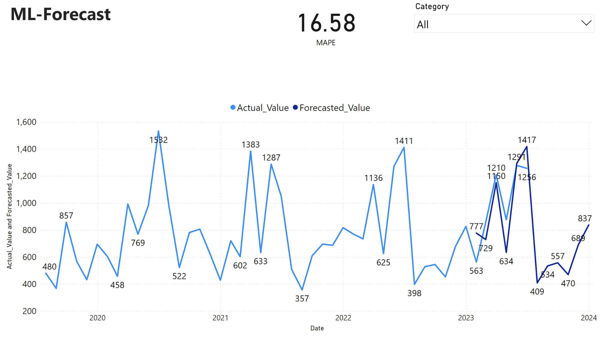
Based on this observation, we can have confidence in the forecasting capabilities of the model for the overall sales in the last six months of 2023, and extending into 2024. This confidence can inform strategic decisions about inventory management, procurement of raw materials, and other business-related considerations.